Packet Centroids of the Riemann Zeta Function
A Smoothing Identity and a Displacement Sum Rule
The framework and the census. Partial sums of ζ travel in packets; each packet's centroid misses ζ by a computable amount. Two theorems, a seven-window census, and the spacing statistics that started everything.
Read this as a workbench
This site is a record of a workbench, not a record of finished results. Rigorous standards were applied to the arXiv paper alone. The paper below is the project's own text, complete — including the negative results, the priority concessions and the errata.
Packet Centroids of the Riemann Zeta Function: A Smoothing Identity and a Displacement Sum Rule
Ondřej Dvořák1
1Independent researcher, Děčín, Czech Republic. on.dvorak@email.cz
AI models used: Anthropic Claude, OpenAI ChatGPT, Google Gemini, xAI Grok.
AI assistance: Large language models were used for computation, proof drafting, proof checking, literature consultation, cross-verification, editing, and manuscript preparation. The mathematical arguments were drafted and checked by these models, including repeated blind refereeing by independent model instances; the author has not independently verified every proof. The author originated and directed the research programme, made the methodological and editorial decisions, reviewed the manuscript, and accepts responsibility for presenting this material. The work is written so that every claim can be checked from what is printed and deposited, without trust in either the author or the models.
Record of work: These files are a record of work, not a record of results. They include measurements that were later corrected, conjectures that were refuted, and observations that have never been checked against the literature. Every claim is marked with which of those it is.
§1. Discovery and Motivation
1.1 Partial-sum spirals and the packet structure
For s = σ + it in the critical strip 0 < σ < 1, the partial Dirichlet sums SN(s) = ∑n=1N n−s trace a spiral on the Argand plane as N increases. The spiral is not uniform: when N crosses the saddle abscissa xν = t/2πν, the ν-th term of the Fourier expansion of the sawtooth ψ(x) = {x} − 12 appearing in the exact truncation formula (made explicit in §2.2–2.3) passes through a stationary point, and the running sum swings direction. Successive saddle crossings divide the integers into packets: the k-th packet is the interval of integers N between two consecutive crossings at xk+1 < xk.
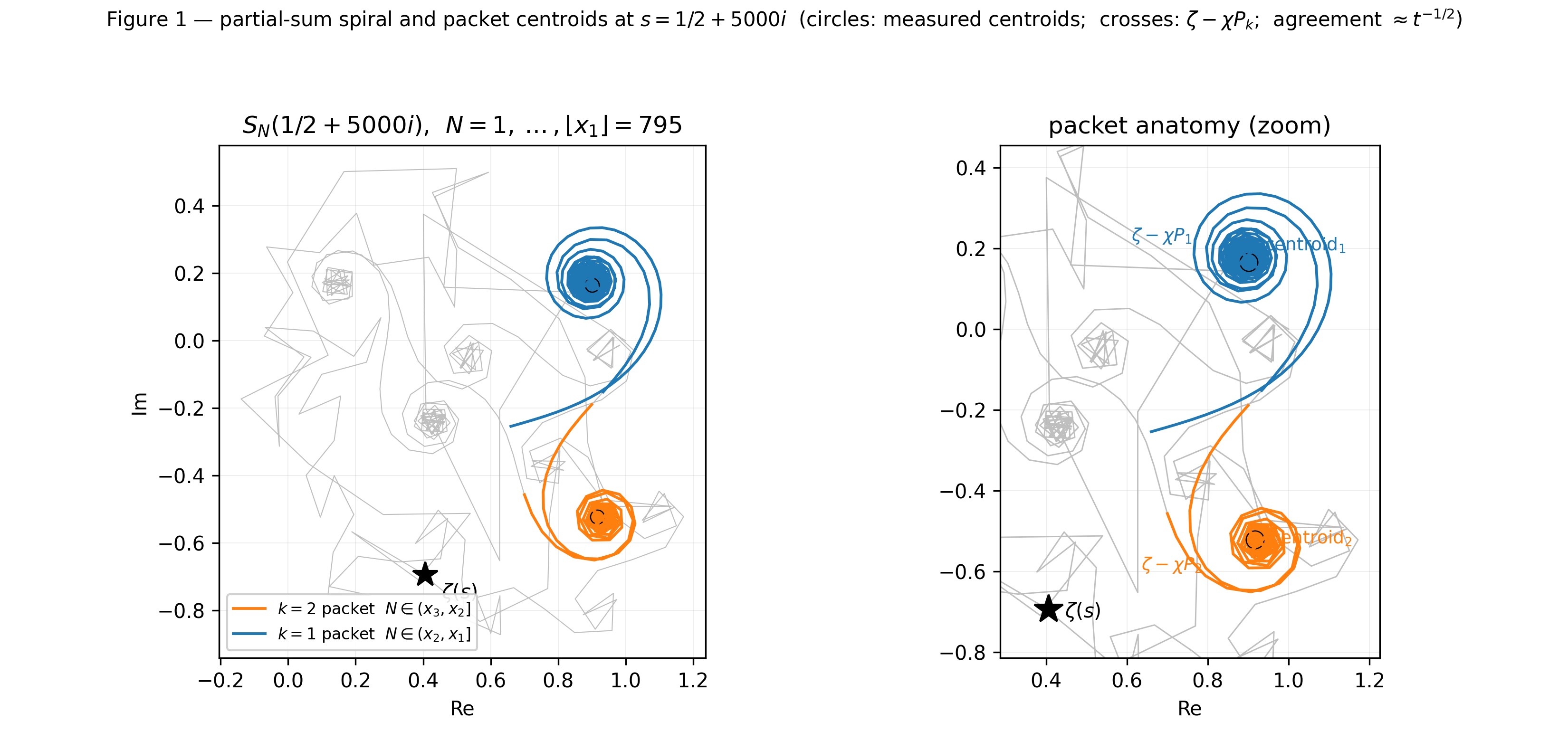
Within each packet the running sum describes a coherent arc — a partial turn of a Cornu-type spiral driven by the single dominant frequency ν = k (Figure 1). The arc terminates and a new arc begins at each saddle. The packet centroid of the k-th arc, and its offset from ζ, are the natural summary statistics: ⟨S⟩k(s) := 1|Gk ∩ ℤ|∑N ∈ Gk SN(s), offk(s) := ζ(s) − ⟨S⟩k(s), where Gk = (xk+1, xk) and the sum is the uniform average over all integer truncation points in the gap. (For the proof in §2 we use a smooth weight supported in the middle third of Gk; Lemma 2.2 in §2 reconciles the two.)
A computation at any s in the strip reveals a striking fact: offk(s) is χ-proportional with a k-term leading expression, and its deviation from that expression decays like t−1/2 (relative to χ) as t → ∞, with oscillating phase. More precisely:
Theorem 1 (§2): For fixed k ≥ 1 and compact [σ0,σ1] ⊂ (0,1), offk(s) = χ(s)Pk(s) + χ(s) Ok,ε(t−1/2+ε), where Pk(s) = ∑m ≤ k ms−1 and χ is the functional-equation factor (defined explicitly in §2.1).
The centroid offset is not zero; it equals χ(s)Pk(s) to leading order — a sum of k terms with χ-proportional weight. Equivalently, the centroid itself satisfies ⟨S⟩k(s) = ζ(s) − χ(s)Pk(s) + χ(s) O(t−1/2+ε). The level-2 zeros — the zeros of the centroid ⟨S⟩k itself — are thus the zeros of ζ(s) − χ(s)Pk(s), which by the functional equation are the points where ζ(w) = Sk(w) in the reflected variable w = 1−s = (1−σ) + it.
1.2 From spirals to value distribution
The map s ↦ w = (1−σ)+it sends the critical strip to itself and converts the geometric question — where does the centroid nearly vanish? — into a question in the analytic theory of the Riemann zeta function: for which w in the strip does ζ take the value Sk(w)?
For k=1, S1(w) = 1: the roots are the 1-points of ζ, studied since Levinson [1] and carrying a known mean density (1/2π)log(t/4π) per unit height (the classical a-point density, distinct from ζ's own zero density (1/2π)log(t/2π); §3.4 uses the former to rescale the k-family gaps and the latter for the Riemann-zero control). For k ≥ 2, Sk(w) = 1 + 2−w + ⋯ + k−w varies with position, and the root family is new. Throughout, write Fk(w) := ζ(w) − Sk(w) for the comparison function; the roots in question are the zeros of Fk.
Two features of the root distribution emerge from a high-precision census:
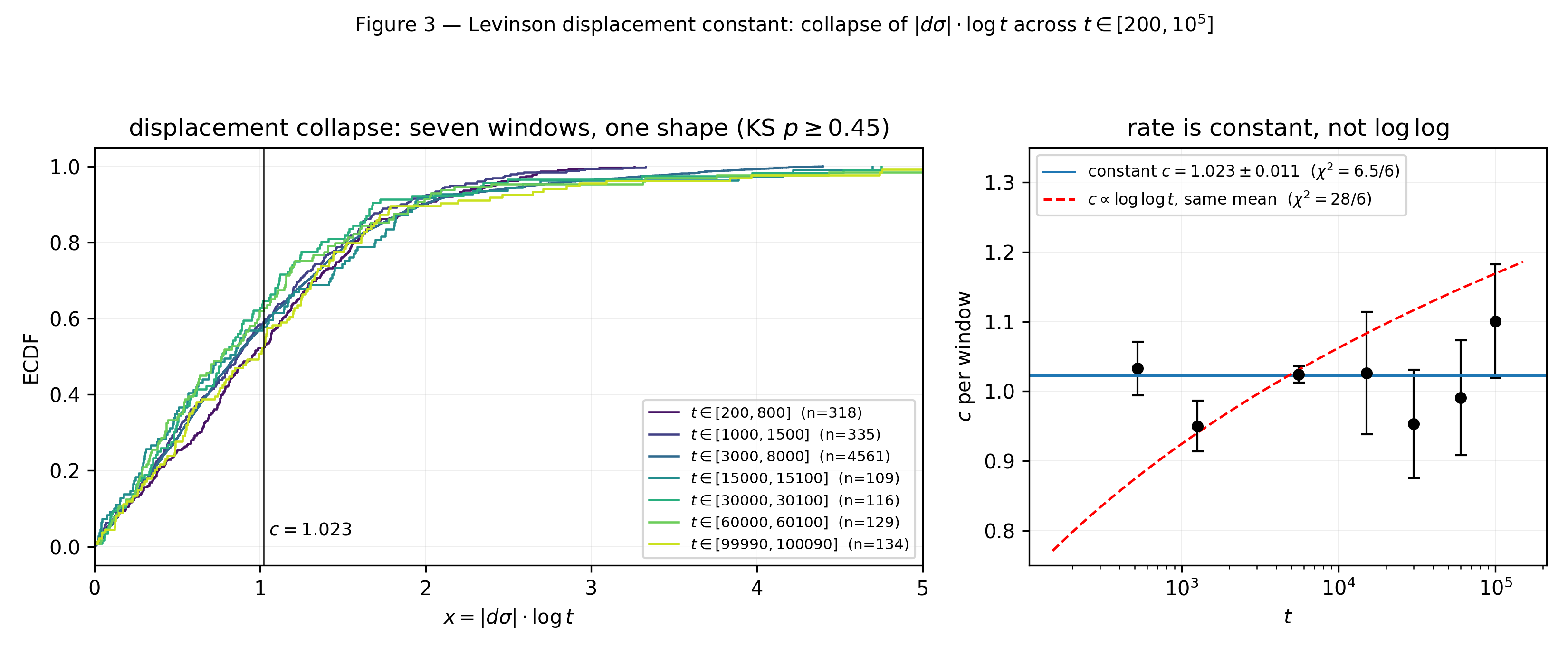
(a) Displacement rate. Each root wρ = uρ + ivρ lies at signed displacement dσρ := σ*ρ − 12 = 12 − uρ from the critical line — the sign convention of the census, positive on the side σ* > 12, i.e. uρ < 12; note that u = 1 − σ* makes uρ − 12 and dσρ opposite in sign. The product |dσρ| · log vρ has a distribution that collapses (KS p ≥ 0.45) to a common shape across heights from t = 200 to t = 100,040, with mean c = 1.023 ± 0.011. This constant is a finite-T analogue of Levinson's clustering rate, here measured directly from the 1-point locations.
(b) Displacement asymmetry. The mean displacement from 12, signed by uρ − 12, is positive and grows like log(k+1): Dk(T1,T2) := ∑Fk(wρ)=0 , vρ ∈ (T1,T2] (uρ − 12) = T2−T14πlog(k+1) + Ok(log T2). (The sum rule's natural variable is uρ − 12 = −dσρ; the positive budget Dk > 0 thus means that the net displacement lies on the side dσ < 0.)
Proposition 2 (§4) proves this law from Littlewood's lemma. The proof reveals that the comparison function H(w) = χ(w)Fk(1−w) appearing on the left of the Littlewood integral equals ζ(w) − χ(w)Pk(w) — exactly the centroid's leading expression, i.e. ζ minus Theorem 1's main term. The smoothing lemma and the sum rule thus share a single object; their derivations are two views of the same asymptotic identity.
1.3 Figures
The paper's five figures are collected in the companion volume Packet Centroids: Visuals [16], with the data behind each. They are cited in the text as Figure 1 ... Figure 5.
§2. The Smoothing Lemma
What Theorem 1 is (added 2026-09-04). Theorem 1 is the Hardy–Littlewood approximate functional equation — Titchmarsh, The Theory of the Riemann Zeta-Function, Theorem 4.16 — specialised to the case 2π xy = t with the cutoff x = N placed inside the k-th saddle gap Gk, so that the reflected sum is exactly Pk. The two standard inputs of the derivation below, Poisson summation and stationary phase, are its standard inputs and are cited as such (Titchmarsh ch. IV). What is this paper's own is the remainder and the transfer: the error O(k/√t) relative to χ for a cutoff held away from the saddles, the bounded oscillating factor Φk carried rather than absorbed, and the passage from the smooth-weight statement to the uniform packet centroid (Remark 2.2). A reader who knows the approximate functional equation should read §2 as a sharpened remainder for an interior cutoff, not as a new identity.
Theorem 1. Fix k ≥ 1, a compact [σ0,σ1] ⊂ (0,1), and ε > 0. Then, uniformly for σ ∈ [σ0,σ1], offk(s) = χ(s)Pk(s) + χ(s) Ok,σ0,σ1,ε(t−1/2+ε), where the error, written as χ(s) t−1/2 Φk, carries an oscillating factor Φk ≪k,ε tε whose dominant part has phase depending on {t/2π k} and {t/2π(k+1)} (§2.5).
2.1 Setup and notation
Write xν:=t/2πν for the ν-th saddle abscissa and let Gk:=(xk+1, xk), |Gk|=t2π k(k+1), be the k-th packet gap. Fix a weight ω∈ Cc∞(Gk), suppω contained in the middle third of Gk, ∫ω=1, ω(j)≪j|Gk|−j, and set the discrete normalization ω(N)=ω(N)/∑M∈ℤω(M). The smooth-weight centroid offset of §2 is offk(s) = ζ(s) − ∑Nω(N) SN(s) = ∑Nω(N) TN(s), TN(s):=∑n>Nn−s, the tail TN being defined for 0<σ<1 by analytic continuation from σ>1 (equivalently Abel regularization); all identities below are exact identities of the continuations. Here χ(s) = 2sπs−1sin(π s/2) Γ(1−s) is the functional-equation factor, with the Stirling asymptotic χ(s) = (2π/t)s−1/2ei(t+π/4)(1+O(1/t)) as t → ∞, uniformly on compact σ-sets; its zeros and poles all lie on the real axis.
2.2 Step 1 — exact truncation formula
For integer N≥1 and σ>0, Stieltjes integration of x−s against d⌊x⌋=dx−dψ(x), ψ(x):={x}−12, gives the exact formula TN(s) = N1−ss−1(a) smooth term − 12 N−s(b) local term − s∫N∞ ψ(x) x−s−1 dx(c) ψ−integral . Terms (a) and (b) are error-sized relative to χ: with N≍ t/k, |N1−s/(s−1)||χ(s)|≍ kσ−1t−1/2, |N−s||χ(s)|≍ kσ t−1/2, both uniform on [σ0,σ1]. Every main term therefore comes from (c).
2.3 Step 2 — Poisson expansion of the ψ-integral
Insert ψ(x)=−∑ν≥1sin 2πν xπν into (c): (c) = ∑ν≥1s2π iν∫N∞ (e(ν x)−e(−ν x)) x−s−1 dx = ∑ν≥1(Iν(N)−I−ν(N)).
Justification of the interchange (dominated convergence). The termwise integration behind this display holds for each fixed N; no smoothing in N is needed at this step — the ω-average enters only later, in the Fresnel-defect bounds of §2.4–2.5. Let ψV(x):=−∑ν≤ Vsin2πν xπν be the partial sums of the sawtooth series. (i) ψV(x)→ψ(x) at every non-integer x (Dirichlet's convergence theorem for the piecewise-C1 function ψ); the exceptional integers are a null set for dx. (ii) |ψV(x)|≤4 uniformly in V and x: at integer x every term vanishes; otherwise, with \|x\| the distance from x to the nearest integer and ν0:=⌈1/\|x\|⌉, each term with ν≤ν0 is at most 2\|x\| in modulus (from |sin2πν x|≤2πν\|x\|), so these contribute at most 2\|x\|ν0≤2+2\|x\|≤3; for the terms ν0<ν≤ V, the geometric-sum bound |∑ν≤ Me(ν x)|≤1/(2\|x\|) gives |∑ν0<ν≤ Msin2πν x|≤1/\|x\|, and partial summation against the decreasing weights 1/(πν) bounds their contribution by (1/π)·(1/\|x\|)·(ν0+1)−1≤1/π. The dominating function is therefore 4x−σ−1, integrable on (N,∞) because σ≥σ0>0. Dominated convergence gives ∫N∞ψ(x) x−s−1dx=limV∫N∞ψV(x) x−s−1dx, and each ∫N∞ψV x−s−1dx is the finite sum ∑ν≤ V of absolutely convergent integrals. The ν-series in the display is thus summed as the limit of its symmetric partial sums ∑ν≤ V(Iν−I−ν); the estimates below show that the negative-frequency sum and the class-(iii) sum converge absolutely, so no rearrangement issue arises downstream.
The phase of I±ν is φ±ν(x)=±2πν x−tlog x, with φ±ν'(x)=±2πν−t/x. For the negative frequencies φ−ν'≤ −2πν on x>0: no stationary point, and repeated integration by parts yields ∑ν|I−ν(N)|=|χ(s)| Ok(t−1/2) (this bound is input (ii) of the status note at the end of §2.6). The positive frequency ν has the unique saddle xν=t/2πν, φν''(xν)=t/xν2>0.
2.4 Step 3 — saddle classification and endpoint weights
For N∈suppω (middle third of Gk) the saddles split into three classes.
(i) Captured saddles ν≤ k: full weight, and the identity that creates Pk. Here xν≥ xk>N, so the saddle lies inside the integration range at distance ≥|Gk|/3 from the endpoint. Stationary phase at xν with amplitude s2π iνx−s−1 gives, using 2πν xν=t and s/it=1+O(1/t), Iν(N) = xν−σ· xν√2πt ei(t−tlog xν+π/4) (1+Fν(N)+O(t−1)) = (2πt)s−12ν s−1ei(t+π/4)(1+Fν(N)+O(t−1)), and by the standard asymptotic χ(s)=(2π/t)s−1/2ei(t+π/4)(1+O(1/t)), Iν(N) = χ(s) ν s−1(1+Fν(N))+χ(s) O(t−1) (1≤ν≤ k). Fν(N) is the Fresnel-truncation defect: the deficit of the half-line Fresnel integral cut at distance dν=|xν−N| from its critical point, of size (κν dν)−1 with Fresnel scale κν=√φν''(xν)=√t/xν (the size follows from one integration by parts on the Fresnel tail, ∫D∞ eiu2 du = O(1/D); the full expansion with its uniform O(t−1) error is the standard stationary-phase lemma — see the status note at the end of §2.6 and [18], ch. IV). For ν≤ k and N in the middle third, dν≥|Gk|/3, whence |Fν(N)| ≪ xν√t dν ≪ k√t.
(ii) Ejected saddle ν=k+1: weight zero. Now xk+1<N, the saddle lies outside [N,∞) at distance dk+1≥|Gk|/3; only the Fresnel tail survives: Ik+1(N) = χ(s) (k+1)s−1 Fk+1(N) + χ(s) O(t−1), |Fk+1(N)|≪ k t−1/2.
(iii) Distant frequencies ν≥ k+2: |φν'|≥ 2π(ν−(k+1))·(1+o(1)) on [N,∞); non-stationary integration by parts and summation over ν give a total χ(s) Ok(t−1/2) (again input (ii) of the status note, §2.6).
Summing (i)–(iii) and averaging over N with ω: offk(s) = χ(s)∑ν≤ kν s−1 + χ(s) t−1/2 Φk = χ(s) Pk(s) + χ(s) t−1/2 Φk, with Φk ≪k,ε tε — the tε absorbs the unexhibited ν-summation losses, the next-order stationary-phase corrections, and (under the uniform weight) the logarithm of Lemma 2.2; see the status note at the end of §2.6.
Remark 2.1 (endpoint weight wk=1; recovery of the sharp-cutoff "½ + ½" bookkeeping). In the sharp-cutoff picture with truncation placed exactly at the saddle, N=xk, the frequency-k term carries only half the Fresnel mass, Fk→−12, i.e. weight 12. Sweeping the truncation point across Gk restores the missing half over one Fresnel transition width κk−1≍ √t/k, and under the centroid average the endpoint frequencies emerge with weights exactly 1 (ν=k) and 0 (ν=k+1): this is the unit endpoint weight wk=1 of the sharp-cutoff bookkeeping, with the two halves recombined by the average. The geometric verification — Newton on the off2 centroid returning w2=1 with finite-t error 0.067/0.035/0.016 at t≈500/1250/5000 — measures precisely this factor, and its measured decay is the theorem's t−1/2 (fitted exponent 0.504 over 24 heights, t∈[300,60000]).
Lemma 2.2 (Uniform-weight extension). Theorem 1 holds, with the same error order t−1/2+ε, for the literal uniform average over all integers N ∈ Gk — the object measured in §3. Proof (given the Fresnel-defect input of §2.4). The proof above uses the smooth weight ω supported in the middle third of Gk, placing every N at distance ≥ |Gk|/3 from both saddle abscissae and bounding every Fresnel defect by O(k/√t). Under the uniform weight, the endpoint frequencies ν ∈ {k, k+1} see integers at all distances d from the saddle. Integers within the Fresnel transition width κk−1 ≍ √t/k of either endpoint contribute defects Fν(N) = O(1); there are at most O(√t/k) such integers near each endpoint, while the total count in Gk is |Gk| ≍ t/k2, so their share of the average is O(k/√t) · O(1) · χ(s) = χ(s) · O(t−1/2) — the same order as the middle-third estimate. An integer at larger distance d from the saddle carries a defect of size (κk d)−1 = xk/(√t d); averaging over d from κk−1 up to |Gk| costs 1|Gk|∑κk−1 ≤ d ≤ |Gk| xk√t d ≪ xk√t |Gk| log(κk|Gk|) ≪ k√t log t, which is absorbed by the tε of the theorem (and is where that ε is spent under the uniform weight). The interior frequencies are unchanged. ∎ The oscillating prefactor Φk is, under this reading, the t-varying phase of the endpoint integers under the uniform average; the fitted decay exponent 0.504 of Remark 2.1, with its residual ± 0.3–0.4 wobble visible and uncollapsed, measures exactly this uniform-weight object.
2.5 Step 4 — error assembly and the fractional-part wobble
The dominant error is the pair of endpoint Fresnel defects Fk,Fk+1. Their phases are φν(N)−φν(xν)≈12φν''(xν) (N−xν)2 (mod 2π), evaluated at integers N; the offset of the integer lattice from the saddles is exactly {xk}={t/2π k} and {xk+1}={t/2π(k+1)}. Hence Ek(s) = χ(s) t−1/2 Φk(t;{t/2π k},{t/2π(k+1)}), Φk ≪k,ε tε , oscillating. Φk must be carried as an oscillating factor and not absorbed into a smaller power of t: the measured residual wobble of ±0.3–0.4 in log scale is this factor, and any fit forcing a pure power law through it misestimates the exponent.
Forward reference (companion paper). The functional form of Φk — left open here — is the subject of the companion paper [13]: the factor is measured directly, models in the two fractional parts alone are refuted (the factor carries explicit t through the Fresnel scale κν = √t/xν), and a parameter-free Fresnel-endpoint prediction reproduces the measurement with median R2 = 0.993 over k = 1..8, the residual being attributed to instrument artifacts of the prediction. Theorem 1's error term is thereby mechanism-identified, not merely bounded ([13], ch. 3–4). None of this is used in the present paper, and the claim in this paragraph is the companion's, verifiable only once [13] is available.
2.6 Step 5 — uniformity in σ
Every σ-dependence above enters through the bounded continuous factors kσ−1, kσ, the exact ratios xν−σ(t/2π)σ=νσ (in which the σ-dependence cancels against the χ-normalization), and the O(1/t) correction to s/it; on the compact [σ0,σ1] all are uniformly bounded, and the leading stationary-phase constant is σ-independent. Thus the implied constant in O(t−1/2+ε) is uniform on the compact, and the error is χ-proportional with σ-independent ratio. ∎
Numerically, the error/χ ratio varied by ≤5.7% between σ=0.3 and σ=0.5; the specification of this check (window, sample size) is not carried in this paper, and the check is a consistency observation, not part of the proof.
Status of the proof. Two classes of estimates above are used in their standard form rather than proved from first principles: (i) the truncated stationary-phase expansion of §2.4(i)–(ii) — the main-term coefficient with its uniform O(t−1) error, and the Fresnel-tail size (κν dν)−1 — and (ii) the repeated-integration-by-parts bounds, with summation over ν, for the negative frequencies (§2.3) and the distant frequencies (§2.4(iii)), on the infinite range [N,∞). Both are standard applications of the exponential-integral (van der Corput / stationary-phase) lemmas of [18], ch. IV; the hypotheses required there are elementary for the amplitudes s2π iνx−s−1, but the verifications are not written out here, and the tε in the theorem absorbs the unexhibited summation losses (and the logarithm of Lemma 2.2). A reader requiring a fully self-contained proof should treat Theorem 1's error term as resting on these two standard inputs; the main term χ Pk, the error exponent (fitted 0.504 over 24 heights, Remark 2.1), the χ-proportionality, and the oscillating prefactor are each confirmed independently by the census of §3.
Corollary 2.3 (Zero correspondence). Since Fk has real Dirichlet coefficients, Fk(w) = 0 ⇔ Fk(w) = 0. The census records roots wρ = (1−σ*) + it* with t* > 0, i.e. wρ = 1−s for s = σ* + it*. Dividing by χ(s) and applying the functional equation, the zeros of the leading expression ζ(s) − χ(s)Pk(s) at s = σ + it, t > 0, correspond exactly to roots w = (1−σ) + it of Fk(w) = 0. This exact correspondence is what identifies the census population.
The zeros of the centroid ⟨S⟩k itself differ from these by the error term: at a centroid zero, the reflected equation reads Fk(w) = δ(w) with δ := Ek/χ, so |δ| ≪k,ε t−1/2+ε by Theorem 1. If w0 is a simple root of Fk and r > 0 is such that the disk |w − w0| ≤ r contains no other root of Fk and min|w−w0|=r|Fk| > sup|w−w0|≤ r|δ|, then Rouché's theorem gives exactly one zero of the perturbed equation in that disk, and to first order its displacement from w0 is δ(w0)/Fk'(w0). These hypotheses — simplicity, separation, and the lower bound on the circle — are not verified here for the census populations, and they can fail exactly where |Fk'| is small, the regime that drives the displacement statistics of §3.2. The first-order reading |dσ| ≈ |δ|/|Fk'| is therefore a working approximation supported by the measured correlation Corr(|dσ|, 1/|F2'|) = 0.58, monotone from Q1 to Q3 of |F2'| (§3.2) — not a proved bound.
§3. The k-family Census
3.1 Instrument
Roots of Fk(w) = ζ(w) − Sk(w) = 0 are located by Newton's method on a dense grid. The evaluator uses the Euler–Maclaurin formula with N = max(100, ⌈t ⌉) Dirichlet terms and 12 Bernoulli correction pairs, with Kahan-compensated summation; this gives float64 accuracy for t ≤ 60,000 and approaches the double-precision floor (∼ 10−10) near t = 105. The Newton grid has step sizes Δ t = 0.5, Δ u = 0.2 in the primary box u ∈ [−0.5, 1.5]; duplicate roots within tolerance 10−4 in both coordinates are merged. Before each census window, the evaluator is validated against a reference table (15/15 value matches, 12/12 Newton convergence on the low-range table; 12/12 and 12/12 on the high-range table; both tables and their coverage are recorded in the Supplementary Materials [15], §S3). The census dataset was frozen on 2026-07-08.
The strip family consists of roots with u ∈ [0,1] (equivalently σ* ∈ [0,1]); roots with u > 1 (σ* < 0) form the ROS family (Reflected-Outer-Strip), which extends to u ≤ u*(k) as established in Lemma 4.1.1. The initial census box reached u ≤ 2.0 and therefore truncated the high-u ROS tail; the repaired window u ∈ [1.4, k+2.1] is proved complete on the right by Lemma 4.1.1(1). See §4.2 for the census window and its completeness; the record of the repair is in the Supplementary Materials [15], §S1.
3.2 Windows and the Levinson displacement constant
Seven strip windows were surveyed for k = 1 (F1(w) = ζ(w) − 1 = 0, the 1-points of ζ):
| window | n (strip) | tmid | $c = \langle | d\sigma | \cdot \log t \rangle$ |
|---|---|---|---|---|---|
| [200, 800] | 318 | 520 | 1.033 | ||
| [1000, 1500] | 335 | 1255 | 0.950 | ||
| [3000, 8000] | 4561 | 5570 | 1.024 | ||
| [15000, 15100] | 109 | 15051 | 1.026 | ||
| [30000, 30100] | 116 | 30050 | 0.953 | ||
| [60000, 60100] | 129 | 60050 | 0.991 | ||
| [99990, 100090] | 134 | 100040 | 1.101 |
The normalized displacement xρ = |dσρ| · log tρ* has a distribution that collapses across all windows (Figure 3; Kolmogorov–Smirnov p ≥ 0.45). Fitting a constant model gives c = 1.023 ± 0.011 (χ2/dof = 6.46/6), consistent with c independent of t (the highest-t window sits nearest the evaluator's stated precision floor, §3.1, and carries this fit's largest single value; that proximity has not been separately ruled out as a contributor). A free-exponent fit yields α = 0.954 ± 0.090, consistent with α = 1 at 0.5σ. The loglog-growth model c ∝ loglog t is rejected (χ2/dof = 28.05/6 against 6.46/6 for the constant model — the model comparison is these two fits). Within the measured range above, the displacement rate is constant; §6.2(a) records its asymptotic status.
For k = 2 and k = 3, the constant increases mildly: at t ∈ [1000,1500], c(k=2) = 1.079 ± 0.046 and c(k=3) = 1.197 ± 0.049. The increase is mechanically explained by the distribution of |Fk'(w)| across the strip: the displacement |dσ| is proportional to 1/|Fk'(w)| at first order (Corollary 2.3), and a regression of |dσ| on 1/|F2'| over the k=2 census confirms Corr(|dσ|, 1/|F2'|) = 0.58 with a monotone decrease from Q1 to Q3 of |F2'|. The variation of c with k is not a new free parameter but a consequence of the varying derivative landscape.
3.3 Displacement split and the sum rule
The signed split of roots across the critical line u = 12 is diagnostic. For k = 1, the strip-family fraction with u > 12 is 49.3% (z = −1.01, p = 0.31), consistent with 50/50 at all windows individually and pooled. For k = 2, the fraction with u > 12 is 54.9% (z = 6.3, p = 3.7 × 10⁻¹⁰) — equivalently, 45.1% of the σ*-values exceed 12. This is a highly significant departure from symmetry.
Proposition 2 (§4) predicts and explains both. The total signed displacement Dk = (Δ T/4π)log(k+1) grows with k while the ROS family's capacity to absorb the budget — the ROS points each contribute uρ − 12 ≈ 1.2–2.0 — is limited by the ROS vertical spacing 2π/logk+2k+1 (one root per ≈15.5 units of height at k=1; per ≈21.8 at k=2) — a heuristic two-term scale, not a derived density; its origin and unproved status are recorded in Remark 4.1.5, and the ROS displacements entering the closure accounting of §4.2 are measured roots, independent of it. At k=1, the ROS family absorbs ∼71\% of D1, leaving the strip nearly balanced. At k=2, the ROS capacity is sparser relative to the larger budget, and the strip inherits a positive remainder — the observed right-bias.
3.4 Spacing statistics
Nearest-neighbor gaps Δ tρ between consecutive strip-family roots (sorted by vρ), rescaled by the local mean density of the respective family — (1/2π)log(t/2π(k+1)), i.e. (1/2π)log(t/4π) at k=1 and (1/2π)log(t/6π) at k=2, and (1/2π)log(t/2π) for the Riemann-zero control — are strikingly sub-Poissonian and sub-GUE. All rows of the table below are computed on the single window t ∈ [3000,8000] — the same window used for the control, so that the comparison is like-for-like — with the density evaluated at the earlier endpoint of each gap and the first gap of the window dropped (n = 4559 gaps at k=1, 4173 at k=2, 5359 for the control):
| distribution | frac < 0.5 | std | frac > 2 |
|---|---|---|---|
| Poisson | 0.394 | 1.000 | 0.135 |
| GUE, exact (Gaudin) | 0.1131 | 0.4243 | 0.0177 |
| Riemann zeros (k=0) | 0.0896 | 0.395 | 0.014 |
| 1-points (k=1) | 0.0160 | 0.362 | 0.014 |
| k=2 family | 0.0201 | 0.369 | 0.0098 |
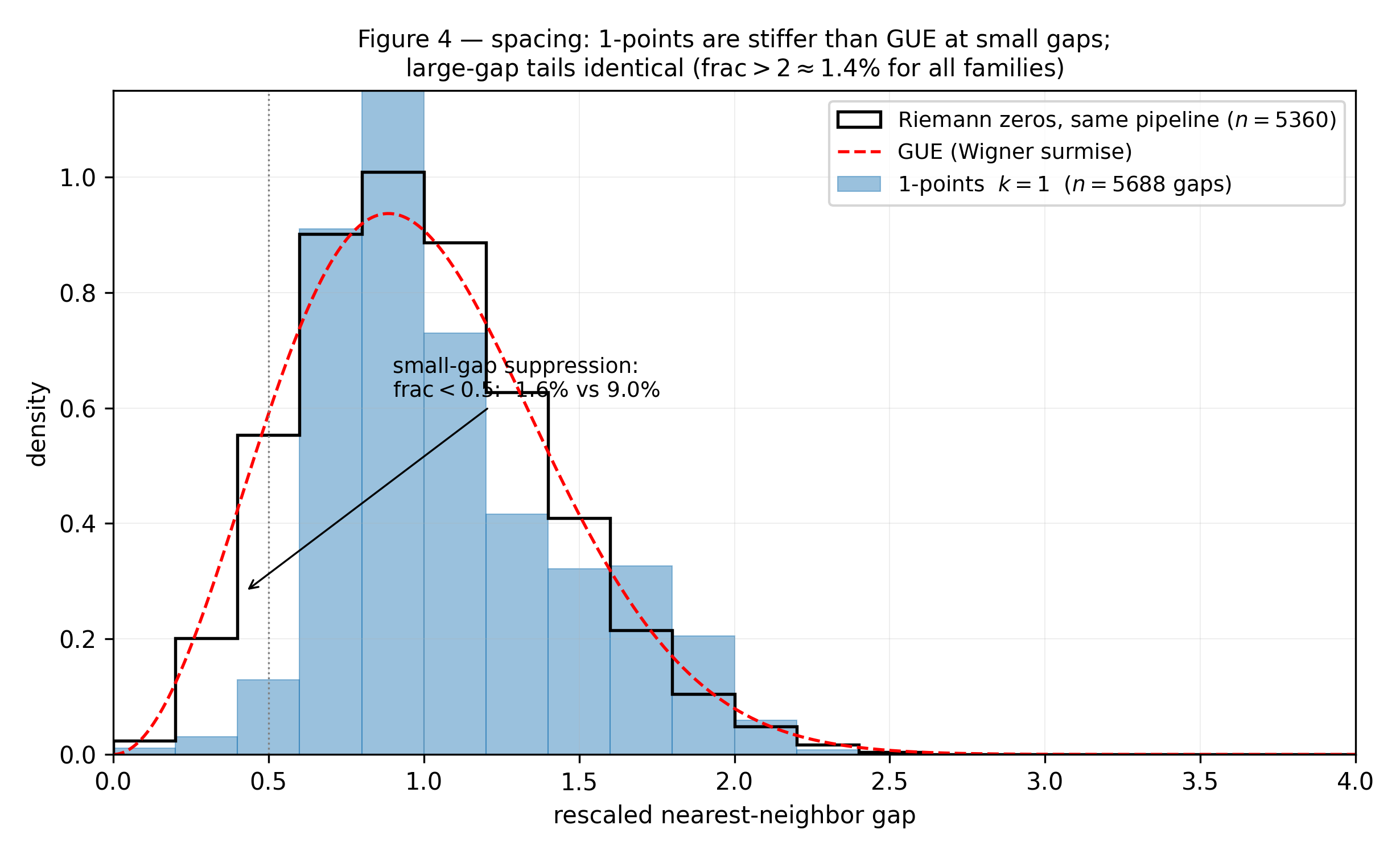
The control uses Riemann zeros in t ∈ [3000,8000] processed on the identical pipeline (same normalisation, same boundary trim). The control is not GUE-consistent, and that is an expected finite-height effect rather than a defect of the pipeline: against the exact row above it carries a small-gap deficit of 20.8% (0.0896 against 0.1131) and an upper-tail deficit of 22.1% (0.0138 against 0.0177), with a standard deviation 7.0% narrower (0.395 against 0.4243). Deficits of the same size at both ends together with a narrower spread are the signature of a distribution compressed relative to GUE, not of a small-gap-specific anomaly; at t ∼ 5×10³ the zeros of ζ are not expected to have reached the GUE limit. The control is therefore an empirical reference at this height, not a stand-in for GUE, and the two comparisons are reported separately below and never merged. The 1-points at k=1 are stiffer than the control by a factor of 6 in small-gap suppression, and at k=2 by a factor of 4.5 — both factors are measurement against measurement and are unaffected by the correction to the reference row. The large-gap tail (frac>2) is indistinguishable between the k=1 family and the control (0.0140 against 0.0138); at k=2 it is 0.0098, below both the control and the exact GUE value (0.0177), from which it is a 45% deficit. The small-gap deficit is therefore the dominant anomaly at both indices, and it is not accompanied by a compensating excess in the upper tail. The pooled seven-window value of frac<0.5 at k=1 is 0.0165; Figure 4 (in the companion Visuals volume) is drawn on that pooled set (n = 5688) and is therefore a different population from this table — both are correct. A diagnostic on the normalisation: the mean rescaled gap, which a correct density constant should place near 1, reads 1.074 at k=2 on this table's constant. (This subsection was corrected on 2026-07-31; the revision record, with the superseded values, is in the Supplementary Materials [15], §S1. It was corrected again on 2026-08-04: the reference row printed 0.090 / 0.42 / 0.010, which are not GUE values — 0.090 was this table's own empirical control restated. The exact Gaudin values are computed by Nyström evaluation of the sine-kernel Fredholm determinant, stable to ten digits over quadrature orders 40–240: F(0.5) = 0.11305539, 1−F(2) = 0.01771044, std = 0.42425685. Every sentence calibrated against the wrong row is rewritten above. No suppression factor and no conclusion of this paper changes, all of them being measured against the control.)
Two artifact checks were passed: (i) refining the seed grid from Δ t = 0.5 to 0.25 at t ∈ [1000,1500] left frac<0.5 unchanged (Δ = 0.0000) and found zero extra strip points; (ii) the Riemann-zero control, computed on the same pipeline, reproduces the published empirical spacing statistics for ζ's zeros at this height. It does not reproduce the exact GUE values, and is not claimed to (see the paragraph above).
Whether this stiffness is known for a-point families with |a| > 1 is an open literature question (see §6).
3.5 Distributional moments and autocorrelation
The distribution of x = dσ · log t (signed displacement times log t, with the sign convention of §1.2: dσ = σ* − 12 = 12 − u) has negative skew throughout: pooled skew −0.713, with ∼40\% attributable to boundary points near u → 1 (σ* → 0, where dσ → −12). After trimming u > 0.9, the residual pooled skew is −0.443, statistically significant in the large windows and growing at high t (caveat: small n at t > 15000). The left tail of dσ is heavier: more roots lie with σ* far below 12 — equivalently uρ far above 12 — than the reverse. This is the same side as the sum rule's budget: Dk > 0 means net displacement at u > 12, i.e. dσ < 0 (§1.2).
The pooled weighted autocorrelation function of dσ (ordered by tρ*) at lag ℓ=5 is −0.077 (3σ outside the white-noise band ±0.026); lags 1–4 are within the band. Consistent with the spacing stiffness: level repulsion produces negative serial correlation at longer lags. A multiple-comparisons correction is required before interpreting the lag-5 value as individually significant.
§4. The Littlewood Displacement Sum Rule
4.1 Proposition 2 (Littlewood sum rule) — full derivation
Standing assumptions. k≥1 fixed; 2π(k+2)≤ T1<T2=:T. Roots are the zeros ρ=uρ+ivρ of Fk(w)=ζ(w)−Sk(w), strip family and ROS family together. Define Dk(T1,T2):=∑Fk(ρ)=0, vρ∈(T1,T2](uρ−12).
Proposition 2. Dk(T1,T2) = T2−T14π log(k+1) + Ok(log T2).
4.1.1 Right normalization and analytic confinement
Lemma 4.1.1. Let G(w):=(k+1)wFk(w). For u>1, G(w) = 1 + ∑m≥ k+2(k+1m)w, |G(w)−1| ≤ Σk(u):=∑m≥ k+2(k+1m)u. Σk is continuous and strictly decreasing on (1,∞) with Σk(1+)=∞, Σk(∞)=0; let u*(k) be the unique solution of Σk(u)=1. Then:
- (Confinement.) Fk has no zeros with u>u*(k). Numerically u*(1)=2.424, u*(2)=3.118, u*(3)=3.811 (computed by bisection on Σk(u)=1 to six significant figures; the displayed values are truncated).
- (Right anchor.) ∫T1T2|log|G(B+it)|| dt≤ 2(T2−T1) Σk(B)→0 as B→∞, uniformly in T1,T2; and |G(B+it)−1|≤12 for all B≥ u*(k)+ck, where ck is the least c ≥ 0 with Σk(u*(k)+c)≤12 (finite, since Σk is continuous and strictly decreasing to 0).
Proof. The series identity is the Dirichlet expansion of Fk for u>1 (valid by absolute convergence of the Dirichlet series for Re(w) > 1); the bound is the triangle inequality; Fk(w)=0 forces |G−1|≥1, i.e. Σk(u)≥1, i.e. u≤ u*(k); (2) is |log(1+z)|≤2|z| for |z|≤12. ∎
Remark 4.1.1-bis (asymptotics of u*(k)). Numerically, u*(k)−k decreases by a near-constant increment per unit k (−0.3061 to −0.3068 over k=1,…,12, converging to ln2−1=−0.306853… by k≈30). This matches the heuristic asymptotic u*(k)∼(k+1)ln2: writing K=k+1 and u=cK, the geometric limit of Σk(cK) as K→∞ is 1/(ec−1), so Σk=1 forces c=ln2 at leading order (the O(1/K) correction is not bounded rigorously). The sharp numerical confirmation is in the per-unit-k increment just quoted: −0.3061 at k=1 is already within 0.3% of the limit ln2−1, reaching 4–5 significant figures by k≈12–30; the bare comparison of u*(k) with (k+1)ln2 is only the leading-order heuristic (1.386 against the true 2.424 at k=1), the relative gap narrowing like 1/k. The confinement bound crosses u=k between k=5 and k=6 (directly computed: offsets +0.198 and −0.109; interpolated crossing ≈5.64). None of this affects the proof, which uses u*(k) exactly; numerics in §4.2 use k≤3.
4.1.2 Left normalization: the reflected comparison function
Lemma 4.1.2. Let H(w):=χ(w) Fk(1−w). Then:
- H(w)=ζ(w)−χ(w)Pk(w) (the centroid's leading expression: the reflected comparison function of the sum rule is ζ minus the smoothing-lemma main term, i.e. ⟨S⟩k to leading order).
- H is analytic on {u≥12, T1<v≤ T2} (the pole of ζ at w=1 and all zeros/poles of χ lie on the real axis), and χ is non-vanishing there; hence the zeros of H in that half-strip are exactly w=1−ρ for roots ρ with uρ<12 (the reflection ρ↦1−ρ preserves the ordinate vρ; since Fk has real Dirichlet coefficients, ρ is a root whenever ρ is, so conjugation is an involution on the root set and the multiset of real parts is unchanged), with Rew−12=12−uρ.
- (Line identity — exact, not asymptotic.) |H(12+it)|=|Fk(12+it)| for all t, since |χ(12+it)|=1 and Fk(w)=Fk(w) (real Dirichlet coefficients), so |Fk(12−it)|=|Fk(12+it)|.
- (Right anchor.) For u=B and t∈(T1,T2]: |H(B+it)−1|≤ 2 1−B+(t/2π)1/2(2π k/t)B(1+o(1)), which is ≤12 once B≥ B0(k,T1) — a threshold independent of T2, and nonincreasing in T1, so that B0(k) := B0(k,2π(k+2)) serves for every admissible T1 — and ∫T1T2|log|H(B+it)||dt→0 as B→∞. In particular every root satisfies uρ≥1−B0, so the left family is finite and fully captured for B≥ B0.
Proof. (1): Fk(1−w)=χ(1−w)ζ(w)−∑m≤ kmw−1; multiply by χ(w) and use χ(w)χ(1−w)=1. (2): χ(w)=2wπw−1sin(π w/2)Γ(1−w) has zeros at even integers and poles at positive integers, all real. (4): Write H−1=(ζ(w)−1)−χ(w)Pk(w) and bound the two pieces on u≥3, t∈(T1,T2]. Dirichlet tail: |ζ(B+it)−1|≤∑n≥2n−B≤2−B+∫2∞ x−Bdx=2−B(1+2B−1)≤21−B for B≥3. Second piece: |Pk(B+it)|≤∑m≤ kmB−1≤ kB, and the Stirling asymptotic |χ(B+it)|=(t/2π)1/2−B(1+O(1/t)) — valid as t→∞ at fixed B, which is the regime of the displayed (1+o(1)) — gives the stated two-term bound by the triangle inequality. The two claims that need uniformity in B (the threshold B0 and the vanishing of the anchor integral as B→∞) we derive instead from an unconditional bound. The reflection formula rewrites the definition of χ as χ(w)=2w−1πw/(cos(π w/2) Γ(w)); for u≥3 and t≥ T1≥2π(k+2) we have |cos(π w/2)|≥sinh(π t/2)≥0.49 eπ t/2, while writing u=x+m with x∈[2,3), m=⌊u⌋−2, the recursion |Γ(u+it)|=|Γ(x+it)|∏j=0m−1|x+j+it|≥|Γ(x+it)| (⌊u⌋−1)! and Stirling on the fixed strip x∈[2,3] (|Γ(x+it)|≥ c0 t3/2e−π t/2, c0 absolute, t≥6π) give, with an absolute constant C, |χ(u+it) Pk(u+it)| ≤ C (2π k)⌊u⌋+1t3/2 (⌊u⌋−1)! (u≥3, t≥ T1), a bound that decreases geometrically at successive integers once ⌊u⌋≥4π k and tends to 0 super-exponentially, uniformly in t≥ T1 and in T2. Choose B0=B0(k,T1)≥3 so that this bound is ≤14 for all u≥ B0 (the displayed bound is decreasing in t, so the choice made at T1 = 2π(k+2) serves for every larger T1: B0 may be taken to depend on k alone); then |H(u+it)−1|≤21−u+14≤12 on {u≥ B0, T1<t≤ T2}, so H≠0 there. Since Fk has real coefficients, a root ρ with uρ<12 and vρ∈(T1,T2] yields the zero 1−ρ of H at ordinate vρ with Re(1−ρ)=1−uρ; hence 1−uρ≤ B0, i.e. uρ≥1−B0, and the left family is finite and fully captured for B≥ B0. Finally, on |H−1|≤12 we have |log|H||≤2|H−1| (as in Lemma 4.1.1(2)), so ∫T1T2|log|H(B+it)|| dt≤2(T2−T1)(21−B+C(2π k)⌊B⌋+1/(T13/2(⌊B⌋−1)!))→0 as B→∞. ∎
4.1.3 Horizontal edges and zero-counting
Lemma 4.1.3. Let Ψ∈{G,H} and B≥ B0.
- |Ψ(σ+it)|≪k tA on [12,B]×[T1,T2] for an absolute constant A (A=1 suffices), uniformly in B; and |Ψ(B+it)|≥12.
- (Edge bound.) Along either horizontal side t=Tj: argΨ(σ+iTj)≪klog T for σ∈[12,u*+1] (resp. [12,B0] for H), while for larger σ, |argΨ|≪Σk(σ) resp. |H−1|, which is integrable in σ uniformly in B. Hence the horizontal contributions to Littlewood's lemma are Ok(log T), uniformly in B.
- (Counting.) NFk(T+1)−NFk(T)≪klog T, where NFk(T) counts the roots with 0 < vρ ≤ T.
- (Contour hygiene.) If a zero of Fk lies on an edge of the rectangle, translate Tj by at most 1 to a zero-free ordinate; by (3) and by confinement (12<uρ≤ u*(k) on the right of the line by Lemma 4.1.1(1), and 1−B0 ≤ uρ<12 on the left by Lemma 4.1.2(4), with B0 = Ok(1)), each root crossed by the moved edge contributes Ok(1) to the displacement sum, so the induced change in Dk is Ok(log T).
Proof sketch and status. (1): for u≥ u*(k) (resp. u≥ B0 for H), |Ψ−1|≤1 by Lemmas 4.1.1–4.1.2, uniformly in B; on the remaining strip 12≤ u≤ u*(k)+1 (resp. B0), the Dirichlet-polynomial factors are Ok(1), |χ(u+it)|≤1+O(1/t) for u≥12 by Stirling, and |ζ(u+it)|≪ t1/2log t by the classical convexity bound; so A=1 suffices. (2) and (3) are the standard Jensen–Borel–Carathéodory apparatus for functions of polynomial growth in a strip, run from anchor disks centered at u=B+1 (where |Ψ−1|≤12) resp. u=u*+2 (where |G−1|<1): the number of zeros of ReΨ on a horizontal segment of length ℓ on which |Ψ|≤ M is ≪ ℓlog M+1; here M≪k tA by (1) and ℓ≪ u*(k)≪ k, giving the Ok(log T) bounds. This is the argument behind the classical estimates argζ(σ+iT)≪log T and N(T+1)−N(T)≪log T ([18], ch. IX), applied to G and H in place of ζ; we use it in its standard form and do not evaluate the constants — which is why the operating tolerance ± O(log T) of §4.2.4 is a working figure rather than a derived one. (4) is immediate from (3) and the two confinement bounds.
What Proposition 2 is (added 2026-09-04). For k = 1 the statement below is Levinson's displacement sum for the 1-points, and the proof is his, with the constant target replaced by Sk and the normalisation 2−w replaced by (k+1)−w. What is new here is the statement for k ≥ 2, the elementary confinement u*(k), and the census — including the outer family, which carries 71 % of D1 and had not been recovered before. (The exact display in Levinson's paper has not been re-read at first hand; if it carries only the count, the correct wording is "by the method of [1]".) And what Proposition 2 buys the wider programme is coordinates, not an obstruction: it is an equality inherited from the functional equation, so it holds verbatim for the Davenport–Heilbronn-type counterexamples that share that equation and cannot separate them from ζ.
4.1.4 Proof of Proposition 2
Apply Littlewood's lemma to G on RB=[12,B]×[T1,T2] (edges zero-free by Lemma 4.1.3(4)). By Lemma 4.1.1(1) all roots with uρ>12 lie in RB: 2π∑uρ>1/2(uρ−12) = ∫T1T2log|G(12+it)| dt − ∫T1T2log|G(B+it)| dt + Ok(log T), and on the line log|G(12+it)| = log|Fk(12+it)| + 12log(k+1). Apply Littlewood's lemma to H on the same rectangle; by Lemma 4.1.2(2,4) its zeros there are in bijection with all roots uρ<12, with distance to the left edge 12−uρ: 2π∑uρ<1/2(12−uρ) = ∫T1T2log|H(12+it)| dt − ∫T1T2log|H(B+it)| dt + Ok(log T), and by the exact line identity, log|H(12+it)|=log|Fk(12+it)| pointwise.
Subtract the two displays and let B→∞ (both right-anchor integrals vanish by Lemmas 4.1.1(2), 4.1.2(4); the horizontal bounds are uniform in B): 2π Dk(T1,T2) = T2−T12 log(k+1) + Ok(log T2). ∎
Remark 4.1.4 (why the rule is "free"). The two line integrals ∫log|Fk(12+it)| dt cancel identically — no estimate of the line integral, no information about the value distribution of Fk on the line, is used. The entire displacement budget is the normalization asymmetry between the two ends of the strip: (k+1)−w on the right versus χ on the left. Roots exactly on u=12 contribute 0 to both sides (formally: apply Littlewood's lemma on [12+δ,B] and on its reflected counterpart, and let δ→0+; roots on the line contribute 0 in the limit).
Remark 4.1.5 (consequences, restated for §4.2). With Δ T=T2−T1: Dk=(Δ T/4π)log(k+1) gives D1[3000,8000]=275.8, D1[1000,1500]=27.6, D2[3000,8000]=437.1, D2[1000,1500]=43.7, D3[1000,1500]=55.2. The k=1 50/50 strip split is a cancellation special to a=1 (the ROS family at u>1 absorbs essentially all of D1, each contributing uρ − 12 ≈ 1.2–2.0, measured mean 1.244 at k=1 [3000,8000]); for k≥2 the ROS family is sparser (vertical spacing 2π/logk+2k+1: 15.5 at k=1, 21.8 at k=2) while the budget grows like log(k+1), so the strip inherits a positive remainder — the measured 54.9% of k=2 roots with u>12 (z=6.3), equivalently 45.1% with σ*>12.
Status of the ROS spacing scale (heuristic, not proved). For u>1, Fk(w)=∑m≥ k+1m−w=(k+1)−wG(w) with G as in Lemma 4.1.1, and after the constant term the slowest-rotating term of G is ((k+1)/(k+2))w, whose phase completes one revolution over the vertical period 2π/logk+2k+1; one root per revolution of the slowest phase is the generic expectation for such a balance, and that is the sole origin of the quoted scale. It is not a derived density, and we do not prove it: at the relevant u the remaining tail of G is comparable to the (k+2)-term (by the definition of u*(k), the full tail sums to 1 there), so no two-term reduction is available, and an actual asymptotic vertical density for the ROS family would require a mean-motion analysis of the almost periodic function G in the sense of Jessen–Tornehave [17], which we have not carried out. The scale enters this paper only in the mechanism-level reading of the strip/ROS partition, here and in §3.3; every quantitative ROS statement — the closure table of §4.2.4 and the strip/ROS anatomy there — sums measured roots and does not use the formula.
4.2 The census window: analytic confinement and closure
4.2.1 The census box and its cutoff
The original census box was u∈[−0.5,1.5], with an acceptance cutoff at u = 2.0: roots with u>2.0 were excluded. The k-th ROS family, governed at its outer edge by the balance of (k+1)−w against the tail ∑m≥ k+2m−w, reaches further right as k grows, because (k+1)−w decays more slowly in u. The cutoff therefore excluded exactly the high-u, high-displacement points — each carrying u−12≈1.2–2.0 — and excluded more of them at larger k. (The chronology of the defect and its repair is recorded in the Supplementary Materials [15], §S1.)
4.2.2 The analytic confinement window
Lemma 4.1.1(1) makes the repaired window an analytic statement rather than a guess: every root satisfies u≤ u*(k), the unique solution of ∑m≥ k+2((k+1)/m)u=1, with u*(1)=2.424, u*(2)=3.118, u*(3)=3.811, each strictly below the patch ceiling k+2.1 (=3.1, 4.1, 5.1). The patch window u∈[1.4, k+2.1], abutting the original box, is therefore provably complete on the right, with margin. The data agree: observed patch maxima u=1.78 (k=1), 2.47 (k=2), 2.93 (k=3) sit well below both u*(k) and the ceiling — no roots near the ceiling for any k.
| case | patch n | patch u range | mean (u−12) | u*(k) | ceiling k+2.1 |
|---|---|---|---|---|---|
| k=1 [3000,8000] | 6 | [1.71, 1.78] | 1.244 | 2.424 | 3.1 |
| k=2 [1000,1500] | 5 | [2.03, 2.34] | 1.672 | 3.118 | 4.1 |
| k=2 [3000,8000] | 45 | [2.01, 2.47] | 1.656 | 3.118 | 4.1 |
| k=3 [1000,1500] | 11 | [2.12, 2.93] | 1.952 | 3.811 | 5.1 |
4.2.3 Exclusion of an in-box explanation
An alternative explanation of the k≥2 deficits — ∼362 missing in-box roots (near-critical-line points with small |F2'|) — fails on the counting density: the expected in-box count per unit height is 12πlogt2π(k+1), not k-independent. (The k-dependence enters through the leading Dirichlet coefficient (k+1)−w of Fk, exactly as the classical a-point density (1/2π)log(t/4π) [1] reflects the leading coefficient 2−w at k=1; the formula is used here as a counting normalisation, and its asymptotic is not proved in this paper.) Correctly:
- k=2, [3000,8000]: ≈4480 expected vs. 4442 found → ∼38 missing in-box (not 362);
- k=3, [1000,1500]: ≈309 expected vs. 299 found → ∼10 missing in-box.
Near-line stragglers carry mean (u−12)≈0.2: forty of them explain ≈8 of the −74.7 deficit — off by an order of magnitude. The in-box hypothesis is refuted; the deficit had to sit outside the box, in few points of large displacement.
4.2.4 Pre-registration and closure
Proposition 2 fixed the deficits before the patch was run: the sum rule predicted per-window shortfalls of 7.9, 8.3, 74.7, 21.2. The patch census over u∈[1.4,k+2.1] then returned:
| window | patch n | patch Σ(u−12) | predicted deficit | total Σ(u−12) | Dk predicted | residual | % |
|---|---|---|---|---|---|---|---|
| k=1 [3000,8000] | 6 | +7.47 | 7.9 | 275.40 | 275.8 | −0.40 | −0.1% |
| k=2 [1000,1500] | 5 | +8.36 | 8.3 | 43.78 | 43.7 | +0.08 | +0.2% |
| k=2 [3000,8000] | 45 | +74.51 | 74.7 | 436.89 | 437.1 | −0.21 | −0.0% |
| k=3 [1000,1500] | 11 | +21.47 | 21.2 | 55.51 | 55.2 | +0.31 | +0.6% |
The fifth window, k=1 [1000,1500], closed without any patch at −7.3% of D1=27.6 (residual ≈2.0, within an assumed operating tolerance of ± O(log T)≈±10 — the constant in Lemma 4.1.3's bound is not evaluated explicitly, so this is a working figure, not a derived one): consistent, since at k=1 the truncation bites least (u*(1)≈2.4 barely exceeds the old 2.0 cutoff — six roots in 5000 units of height at [3000,8000], and none detectable above noise in the short window).
All five windows close within tolerance; the four patched windows close within 0.6% of Dk. The sum rule closes on all five tested window/index pairs (k = 1, 2, 3).
Strip/ROS anatomy at k=1 [3000,8000]: strip (u∈[0,1]) +79.41; ROS existing +188.52; ROS patch +7.47; total 275.40 vs. D1=275.8. ROS carries 195.99=71.3% of the total. The strip net +79 is real, not ≈0: the sum rule constrains the total displacement, not the strip alone. Roughly 70% of Dk is carried by the ROS family at large u; the strip net displacement is the small positive remainder, consistent with the sum rule constraining the total rather than the strip alone.
Instrument note. Initial census box u∈[−0.5,1.5] (hard cutoff u≤2.0) missed the high-u ROS branch, which is analytically confined to u≤ u*(k)<k+2.1; the patch census over u∈[1.4,k+2.1] recovered 6/5/45/11 roots per window with mean (u−12)≈1.2–2.0, closing all deficits to within 0.6% of Dk. The record of the repair is in the Supplementary Materials [15], §S1.
Summary. (1) Original census: k=1 closes (−2.9%), k≥2 shows 17–38% deficits. (2) Diagnosis: ROS truncation, not in-box incompleteness — the in-box hypothesis fails the counting density by an order of magnitude. (3) Patch census over the analytic confinement window: all deficits recovered, all rows within 1% of Dk, and the recovered u-ranges independently confirm the confinement bound.
The census reported here is final; no further windows were surveyed.
§5. Connection to the Riemann–Siegel Formula
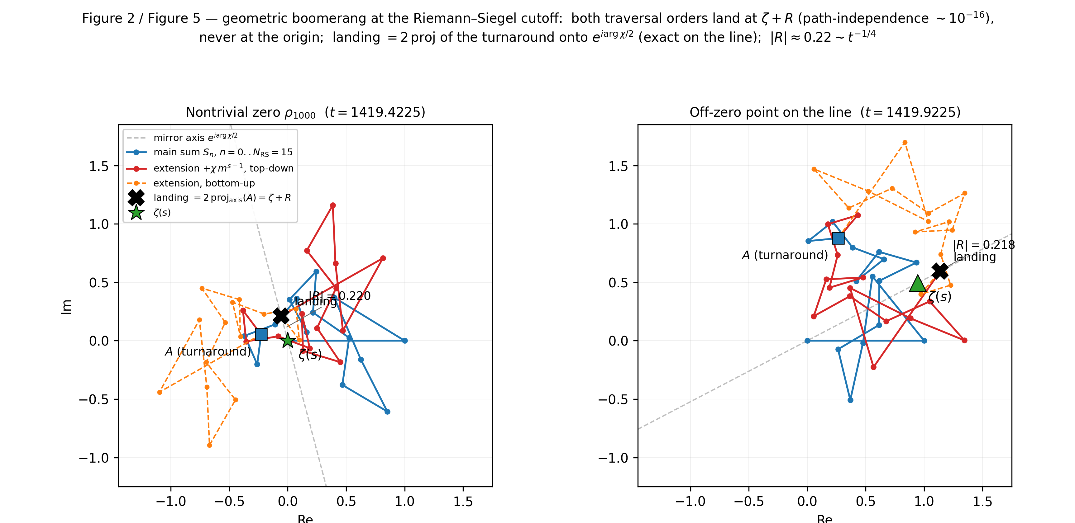
At the Riemann–Siegel cutoff NRS = ⌊√t/2π⌋, the approximate functional equation takes the form ζ(s) = SNRS(s) + χ(s) SNRS(1−s) + R(s), |R(s)| = (t2π)−σ/2 F(p) (1+o(1)), p = {√t/2π}, where F is a bounded, oscillating, σ-independent function of the fractional part p alone, and R is the classical Riemann–Siegel remainder. The σ-dependence of the remainder is the pure power (t/2π)−σ/2, not a bounded prefactor; at σ = 12 this reduces to the t−1/4 rate quoted below. This is the leading term of the classical Riemann–Siegel expansion at general s (Siegel [10]; explicit remainder bounds on the line Gabcke [11]; rigorous general-s formulation Arias de Reyna [12], whose leading coefficient C0 is σ-independent), rediscovered and confirmed at finite height by the boomerang construction — see the Post Scriptum for the measured basis. The boomerang construction (Figures 2 and 5) asks: what happens if we compute the reversed-chirality extension, adding χ(s) SNRS(1−s) to the partial sum SNRS(s)?
Numerically (using Newton-iterated EM ζ, t ∈ [236, 3533]): the construction lands at ζ(s) + R(s), not at 0 or ζ(s). The landing magnitude |R| is ≈ 0.25 at t ≈ 237, 0.22 at t ≈ 1419, 0.10 at t ≈ 3533 — consistent with t−1/4 decay (the σ=12 case of the general law above). The construction is path-independent: traversing the χ-extension top-down vs bottom-up (reversing the order of the NRS terms) reaches the same terminal point to ∼ 10−15 (commutativity of addition). The spiral picture does not "close" at Riemann zeros; the landing misses ζ(s) by |R| ∼ t−1/4 regardless of whether ζ(s) = 0.
On the critical line, the landing has a geometric interpretation: by |χ(12 + it)| = 1 and the real-coefficient symmetry |SNRS(12 − it)| = |SNRS(12 + it)|, the landing vector is 2 projeθ(R) where eθ = ei argχ(12+it)/2. At a Riemann zero, ζ(s) = 0, so |landing|= |R| is the entire displacement from the origin. This is precisely the Riemann–Siegel formula for Z(t) = eiϑ(t)ζ(12+it): the "boomerang" rediscovers it geometrically.
The construction illustrates the second scale at which the geometric picture of §1 encounters classical machinery: at the packet scale (N ∼ t/k) it produces Pk and the smoothing lemma; at the RS scale (N ∼ √t) it produces the RS remainder. The two scales are not in competition — the same truncation-plus-stationary-phase machinery used in §2, applied at the cutoff N ∼ √t/2π rather than N ∼ t/2π k, is the classical route to the approximate functional equation and, pushed to full asymptotic depth, to the RS formula ([10], [12]).
Forward reference (companion paper). A third regime of the same spiral is developed quantitatively in [13]: past the last saddle x1 = t/2π the partial sum SM closes into coils around ζ(s), and on the band M ∈ [2.5 x1, 6 x1] the Euler–Maclaurin tail converges, giving the coil radius in closed form, |SM(s) − ζ(s)| = M1−σ|s−1|·u/2sin(u/2)·(1+O(1/t)), u = t/M, with derived slope-defect constant −0.250778 and winding number −1 per coil at smooth order ([13], ch. 7). The reversed-chirality extension used above belongs to the same instrument family as the winding-number classifiers and the pair-product reality criterion of [13], ch. 8–9.
§6. Scope, Framing, and Open Questions
6.1 What this paper does and does not claim
The paper identifies, proves, and numerically confirms two structural properties of the k-family of partial-sum roots Fk(w) = 0 in the critical strip:
- Theorem 1 (the smoothing lemma): the centroid offset offk equals χ Pk — equivalently, the packet centroid ⟨S⟩k equals ζ − χ Pk — to within a χ-proportional O(t−1/2+ε) error, uniform on compact σ-sets. The proof is via Poisson summation and stationary phase, with two standard exponential-integral estimates used as inputs (the status note of §2.6); the error exponent, the χ-proportionality, and the oscillating prefactor are each confirmed by the census data.
- Proposition 2 (the Littlewood sum rule): the total signed displacement of all Fk-roots from the critical line grows as (Δ T/4π)log(k+1). The proof uses Littlewood's lemma twice, with the key cancellation being the pointwise equality |H(12+it)| = |Fk(12+it)| on the line (Lemma 4.1.2(3)); no estimate of log|Fk| on the line is needed.
The route — geometric/packet/centroid — is, to our knowledge, novel as a starting point for these results. The destinations are classical: the displacement rate c ≈ 1 is a finite-T avatar of Levinson's a-point clustering theorem [1]; the spacing statistics connect to GUE universality in the sense of Montgomery–Odlyzko [4,5]; the sum rule is an application of Littlewood's lemma [6].
The paper makes no claim about the Riemann Hypothesis. The roots of Fk(w) = 0 in the strip are objects distinct from the zeros of ζ(s); their distribution is governed by the sum rule and the smoothing lemma, both of which apply equally whether or not RH holds. The framing is: the geometry of partial sums is a high-precision microscope on the finite-T value distribution of ζ; the mechanisms it exposes are explained by classical theorems, not enforcing them.
Two papers, one finding. This paper and its companion [13] — published with a Supplementary Materials volume [14] — form one two-part, modular finding. The present paper is the framework and the census: the smoothing identity, the sum rule, and the frozen measurements. The companion paper identifies the mechanism of Theorem 1's error term, answers the literature questions of §6.2 (status notes added below), reports its instruments and closure result, and carries the corresponding negative results. The present paper's theorems, proofs, and frozen measurements stand independently: nothing in §1–§5 requires [13] or [14]; the companions are cited at exactly those points where their material is described, not as a dependency of the results themselves.
6.2 Open questions
(a) Is c ≈ 1.02 known? The constant c = ⟨|dσ| · log t ⟩ = 1.023 ± 0.011 governs the displacement rate. Levinson's theorem [1] gives the density of a-points; Selberg's value-distribution results [2] and Steuding's monograph [3, ch. 7] are the closest references. Whether c has an exact closed form or has been previously identified as a universal a-point constant is open. Status (answered in [14], §12.2): the mean displacement law is known and is not a constant — unconditionally ⟨|dσ|⟩·log t ∼ (1/√π)√loglog t (Selberg [2]; Tsang [19]), with no closed-form constant. The statement of record becomes: c = 1.023 ± 0.011 is a finite-height plateau of a quantity whose asymptotic law is 0.564√loglog t (1+o(1)); the census range cannot discriminate the two shapes. The census itself — apparently the first numerical census of a-point displacements at all — the plateau value, and everything at k ≥ 2 have no located counterpart.
(b) Is the sub-GUE stiffness known? The suppression of small gaps by a factor of 6 relative to the Riemann-zero distribution (and GUE) is the sharpest numerical signal in the census. Whether this stiffness is known for the a-point distribution of ζ at any |a| is an open literature question. Status (answered in [14], §12.4, by a failed-search record): no spacing statistics for a-points of ζ — any a, any height, theorem, conjecture, or numerics — were located, nor any a-point pair correlation. The measurement appears to be the first of its kind; the closest analog-in-spirit is the spacing rigidification of ξ'-zeros (Farmer–Gonek; Farmer–Rhoades [20]), whose mechanism does not transfer as stated and does not predict the observed tail identity.
(c) Is the negative skew known? The distribution of dσ · log t (dσ = σ* − 12, the sign convention of §1.2 and §3.5) has residual skew −0.443 after boundary trimming, growing at high t; the measured heavy tail lies on the side σ* < 12, i.e. roots at uρ > 12. This asymmetry is not predicted by the sum rule (which constrains the mean, not the shape) and may reflect the non-symmetric value distribution of ζ in the strip. Status (compared in [14], §12.3): the qualitative one-sidedness has a classical counterpart conditional on RH (Selberg [2]; Tsang [19]: a one-sided Gaussian tail at scale √loglog T/log T on one side of the line, excursions on the other side confined to a strictly smaller scale, with Selberg's conjectured asymptotic split of 3/4 to 1/4), which also anticipates the measured growth of the skew with height. Caution: the classical statements are phrased for the a-point abscissa uρ, while the measured skew is in dσ = 12 − uρ; the identification of the heavy sides under this sign reversal is carried in [14] and is not re-verified here. A qualitative literature comparison at most — not evidence for or against RH, since the present measurement is unconditional. The skewness coefficients themselves, the boundary-trim decomposition, and the lag-5 autocorrelation have no located counterpart.
(d) Partial-sum zero literature. The zeros of SN(s) (partial sums, fixed N) have been studied by Spira [7], Montgomery [8], and Borwein et al. [9]. The objects of this paper are different — roots of ζ(w) = Sk(w), a comparison equation. We note the exact identity Fk(w) = ζ(w) − Sk(w) = ζ(w, k+1), the Hurwitz zeta function at integer parameter k+1: for k=1 the roots are the classical 1-points of ζ (Landau; Levinson [1]), while for k ≥ 2 the zero distribution of ζ(w,α) at integer α ≥ 3 appears to be unstudied — the Hurwitz-zero literature (Davenport–Heilbronn 1936 [21]; Cassels 1961 [22]; Spira 1976 [23]) treats 0 < α ≤ 1, where the phenomenology (zeros dense in σ, including σ > 1) is qualitatively opposite to the critical-line clustering measured here at k ≥ 2 and known at k = 1 by Levinson [1]. Connecting the two families (e.g., via the perturbation Fk(w) = 0 → SN(w) = 0 as N → ∞) is a natural direction. Status (developed in [14], §12.1): the integer-parameter Hurwitz positioning is carried through the literature there; the Fk → SN bridge has no located antecedent and remains open ([13], ch. 14).
6.3 Calibration note
The paper was developed by combining symbolic analysis (proof routes, sum-rule derivation) with a high-precision computational census (root-finding via Euler–Maclaurin Newton). We distinguish: (i) verified mathematical results — Theorem 1 and Proposition 2 with complete proofs; (ii) empirical measurements — the specific numerical constants confirmed at the indicated precision and windows; (iii) structural predictions — the sum rule's deficits were computed and stated before the patch census was run (§4.2.4). The match between those predictions and the census outcomes (≤ 0.6% residuals) is independent confirmation that the census recovers what the proved proposition predicts, rather than a calibration artifact — the proposition's correctness rests on the proof of §4.1, not on this match.
Post Scriptum: the general-σ remainder — measurement and classical identification
An earlier version of this paper stated the §5 remainder as |R(s)| ∼ C(σ) t−1/4 with C(σ) bounded on the strip; the measurement below corrects this, and the revision is recorded in the Supplementary Materials [15], §S1. Over a 300-point band at t ≈ 73850 (t/2π ≈ 11746), the σ-ratio test returned |R|(0.3)|R|(0.5) = 2.55281 vs (t2π)0.1 = 2.5528, |R|(0.7)|R|(0.5) = 0.39173 vs (t2π)−0.1 = 0.3917 (rel-std ≤ 4×10⁻⁵ across the band), and at the strip boundary |R|(0.0)/|R|(0.5) = 10.41227 vs (t/2π)0.25 at band centre = 10.41227, with pointwise deviation ≤ 6.1×10⁻⁷ (n = 300): the exponent is −σ/2 to five significant figures, including at σ = 0. Pooled over all σ-legs and heights (n = 4858, t up to 2×10⁶), the rescaled remainder K := |R|·(t/2π)σ/2 collapses to a function of the single variable p = {√t/2π} alone (Fourier-3 fit R2 = 0.993; σ-uniformity CV 5×10⁻⁸ within t-cells), and arg R is σ-independent to ≤ 0.005 rad. Hence the corrected law displayed in §5: |R(s)| = (t2π)−σ/2 F(p) (1+o(1)), p = {√t/2π}, with F bounded, oscillating, and σ-independent. (The measurements of this Post Scriptum were made with dedicated high-precision probe instruments, separate from the float64 census evaluator of §3.1; the §3.1 precision range does not bound them.)
Only after the measurement was the law identified as classical: it is the leading term of the Riemann–Siegel expansion at general s (Siegel [10]; explicit remainder bounds on the line, Gabcke [11]; rigorous general-s formulation, Arias de Reyna [12]). In [12] the leading coefficient C0(p) is σ-independent by construction — σ enters the coefficient recurrence only from C1 on — so the measured σ-independence of F and of arg R is the classical structure, not a new phenomenon. We claim no priority for the law. What the geometric route contributes is the measurement itself: the −σ/2 power and the single-variable collapse were obtained from the boomerang construction of §5 before the classical expansion was consulted. All critical-line statements of §5 are the σ = 12 case and were unaffected by the correction.
References
[1] N. Levinson, Almost all roots of ζ(s) = a are arbitrarily close to σ = 1/2, Proc. Nat. Acad. Sci. USA 72 (1975), 1322–1324.
[2] A. Selberg, Old and new conjectures and results about a class of Dirichlet series, in Proceedings of the Amalfi Conference on Analytic Number Theory (Maiori, 1989), Univ. Salerno (1992), 367–385.
[3] J. Steuding, Value-Distribution of L-Functions, Lecture Notes in Mathematics 1877, Springer, 2007.
[4] H. L. Montgomery, The pair correlation of zeros of the zeta function, Proc. Sympos. Pure Math. 24, Amer. Math. Soc. (1973), 181–193.
[5] A. M. Odlyzko, On the distribution of spacings between zeros of the zeta function, Math. Comp. 48 (1987), 273–308.
[6] J. E. Littlewood, On the zeros of the Riemann zeta-function, Proc. Cambridge Philos. Soc. 22 (1924), 295–318.
[7] R. Spira, Zeros of sections of the zeta function. I, Math. Comp. 20 (1966), 542–550; II, Math. Comp. 22 (1968), 163–173.
[8] H. L. Montgomery, Zeros of approximations to the zeta function, in Studies in Pure Mathematics: To the Memory of Paul Turán, Birkhäuser (1983), 497–506.
[9] P. Borwein, G. Fee, R. Ferguson, A. van der Waall, Zeros of partial sums of the Riemann zeta function, Experiment. Math. 16 (2007), 21–40.
[10] C. L. Siegel, Über Riemanns Nachlaß zur analytischen Zahlentheorie, Quellen und Studien zur Geschichte der Mathematik, Astronomie und Physik, Abt. B: Studien 2 (1932), 45–80. Reprinted in Gesammelte Abhandlungen, Vol. I, Springer, 1966. English translation: E. Barkan, D. Sclar, arXiv:1810.05198.
[11] W. Gabcke, Neue Herleitung und explizite Restabschätzung der Riemann-Siegel-Formel, Dissertation, Georg-August-Universität zu Göttingen, 1979. DOI 10.53846/goediss-5113.
[12] J. Arias de Reyna, High precision computation of Riemann's zeta function by the Riemann-Siegel formula, I, Math. Comp. 80 (2011), no. 274, 995–1009.
[13] O. Dvořák, Packet Centroids II: The Fresnel Mechanism, Coil Geometry, and Zero Conditions of the Partial-Sum Walk, companion paper, in preparation (2026).
[14] O. Dvořák, Packet Centroids II: Supplementary Materials — Literature Positioning, Negative Results, and the Identity Ledger, companion document (2026).
[15] O. Dvořák, Packet Centroids: Supplementary Materials, companion document (2026).
[16] O. Dvořák, Packet Centroids: Visuals, companion document (2026).
[17] B. Jessen, H. Tornehave, Mean motions and zeros of almost periodic functions, Acta Math. 77 (1945), 137–279.
[18] E. C. Titchmarsh, The Theory of the Riemann Zeta-Function, 2nd ed., revised by D. R. Heath-Brown, Oxford University Press, 1986.
[19] K.-M. Tsang, The Distribution of the Values of the Riemann Zeta-Function, Ph.D. thesis, Princeton University, 1984.
[20] D. W. Farmer, R. C. Rhoades, Differentiation evens out zero spacings, Trans. Amer. Math. Soc. 357 (2005), 3789–3811.
[21] H. Davenport, H. Heilbronn, On the zeros of certain Dirichlet series, J. London Math. Soc. 11 (1936), 181–185.
[22] J. W. S. Cassels, Footnote to a note of Davenport and Heilbronn, J. London Math. Soc. 36 (1961), 177–184.
[23] R. Spira, Zeros of Hurwitz zeta functions, Math. Comp. 30 (1976), 863–866.
Project materials
The complete project — all papers with their supplementary and visual companions, and the data behind them — is available at zeta.pukapasoft.xyz.
This paper is one part of a series. Its own companion files are Packet Centroids: Supplementary Materials [15] (revision record and bibliographic verification) and Packet Centroids: Visuals [16] (the five figures, with the data behind each).
Nothing in this work decides the location of any zero of the Riemann zeta function, and no result here is progress toward a proof of the Riemann Hypothesis.
Figures
4 figures. Each opens with the commentary the paper wrote for it; click a thumbnail for the full-size render.
This file carries every figure of the paper named above, with its caption exactly as the paper states it and the data behind it. No figure computes a mathematical quantity. The paper's own text remains the sole document of record.
Figure 1
Figure 1 (spiral + packet anatomy). The partial sum SN(12 + 5000i) traced on the Argand plane for N = 1 to ⌊x1 ⌋. The k=1 and k=2 packets are shaded; the respective centroids (filled circles) lie at ⟨S⟩k = ζ − offk ≈ ζ − χ Pk.
Figure 2
Figure 2 (boomerang pair, the banked data table). Top-down (solid) and bottom-up (dashed) reversed-chirality extensions of SNRS at Riemann zero ρ1000 (t ≈ 1419). Both traversal orders land at the same terminal point ζ(s) + R(s) (cross), with |R| ≈ 0.22, consistent with (t/2π)−1/4 decay [erratum 2026-07-19, ratified — item 7]. At a non-zero (triangle), the landing shifts to ζ(s) + R(s); the offset from ζ is not small. See §5.
Figure 3
Figure 3 (displacement collapse). The empirical distribution of |dσ|·log t for all census windows, overlaid. Mean c = 1.023 (vertical line); loglog prediction (dashed, scaled to the same mean) has the wrong shape.
Figure 4
Figure 4 (spacing histogram). Rescaled gap density for 1-points (shaded, k=1, n=5688 gaps, the pooled seven-window census) vs Riemann zeros (open histogram, n=5359 gaps, the single window t ∈ [3000,8000]) and GUE curve. Small-gap suppression is the dominant signal; the large-gap tails are identical. (Both are normalised densities, so the shapes are comparable; the counts differ because the two populations are drawn from different height ranges. The table in §3.4 above is computed on the single window for both, and its k=1 small-gap cell therefore reads 0.0160 where this pooled set gives 0.0165 — E-P1D-2.)
Figure 5 (fig2_boomerang (same render as Figure 2))
Figure 5 (boomerang pair): see caption at Figure 2. The key visual point is that the two path shapes are distinct while the endpoint is identical — path-independence made visible.
Note on the figure set
Five captions, four renders: Figure 5 is the Figure 2 render read for a different point, and the paper says so in its own caption. Figure 2's data file is named in the caption itself.
Supplementary materials
The audit layer: how the numbers above were checked, what was corrected, and what is owed to whom.
Open the supplementary materials
This file carries the revision record (§S1), the bibliographic note (§S2), and the evaluator validation tables (§S3) of the paper named above. It contains no mathematics that the paper does not state.
S1. Revision record
Census instrument repair (before the data freeze of 2026-07-08). The original census box u ∈ [−0.5, 1.5] carried an acceptance cutoff at u = 2.0; roots with u > 2.0 were not recorded. The k ≥ 2 sum-rule deficits this produced were at first attributed to ∼362 missing in-box roots near the critical line; that hypothesis fails the counting density by an order of magnitude (paper, §4.2.3) and was withdrawn. The deficit was located in the high-u ROS tail: the patch census over u ∈ [1.4, k+2.1] (complete on the right by Lemma 4.1.1(1)) recovered 6/5/45/11 roots per window and closed all deficits to within 0.6% of Dk (paper, §4.2.4). The per-window deficits had been computed from Proposition 2 before the patch census was run.
2026-07-08. Census data freeze. No roots were added or removed after this date.
2026-07-14 (§5 / Post Scriptum). The §5 remainder was originally stated as |R(s)| ∼ C(σ) t−1/4 with C(σ) bounded on the strip. Measurement corrected this to |R(s)| = (t/2π)−σ/2 F(p) (1+o(1)), p = {√t/2π}; the corrected law was subsequently identified with the leading term of the classical general-s Riemann–Siegel expansion (paper references [10]–[12]). All σ = 12 statements were unaffected.
2026-07-19 (three corrections). (a) §1.2: the 1-point density constant corrected to (1/2π)log(t/4π), the classical a-point density, distinct from the zero density (1/2π)log(t/2π). (b) §2.4, first display of class (i): xν−s corrected to xν−σ (the explicit phase factor already carries e−itlog xν). (c) Remark 4.1.1-bis: the 4–5-significant-figure agreement re-attached to the per-unit-k increment u*(k)−k → ln 2 − 1, not to u*(k) itself (the bare comparison of u*(k) with (k+1)ln 2 is off by ∼75% at k=1).
2026-07-31 (§3.4, three corrections; no conclusion of the paper changes). (a) The gap rescaling previously used one k-independent density (1/2π)log(t/4π) for all k-families, contradicting §4.2.3's k-dependent constant (1/2π)log(t/2π(k+1)); the two agree at k=1 and differ at k=2. The k=2 row was recomputed on the correct constant: frac<0.5 0.0173 → 0.0201, std 0.395 → 0.369, small-gap suppression ×5.2 → ×4.5. Diagnostic: the mean rescaled gap at k=2 reads 1.152 on the old constant and 1.074 on the corrected one. (b) The window scope of the table was unstated: all cells are computed on the single window t ∈ [3000,8000]; the pooled seven-window value at k=1 is 0.0165, and Figure 4 is drawn on the pooled set (n = 5688) — a different population from the table; both are correct and are now labelled. (c) The k=2 entry of the frac>2 column previously read 0.014, the value of the other two rows; that figure had not been computed. On the paper's own pipeline the k=2 value is 0.0312 on the old constant and 0.0098 on the corrected one; the claim that the large-gap tail is "indistinguishable across all families" fails at k=2 on either constant and was withdrawn for that index (it stands for k=1 against the Riemann-zero control). Unaffected: the census itself (7/7 windows), the displacement constant c = 1.023 ± 0.011, the entire k=1 row, the entire control row, the sub-GUE headline, and the ×6 suppression at k=1. The spacing pipeline was subsequently re-run independently and reproduced its archived intermediates exactly.
2026-08-03 (statement-level corrections; no numerical value changed). (a) Lemma 4.1.2(2): the zero correspondence corrected from w = 1−ρ to w = 1−ρ, matching the lemma's own proof of part (4); the displacement bookkeeping Re w − 12 = 12 − uρ is unchanged, since real coefficients make conjugation an involution on the root set. (b) Corollary 2.3 restated: the exact correspondence is scoped to the zeros of the leading expression ζ − χ Pk; the perturbation step is stated as Rouché's theorem with explicit hypotheses (simplicity, separation, lower bound on the circle), which are not verified for the census populations; the first-order displacement reading is reclassified as a working approximation. An empirical anchor ("52-pair displacement test r = 0.794") whose specification is carried in no file of this set was removed pending specification. (c) The sign convention of dσ fixed as dσ = σ* − 12 = 12 − u (the convention of the census data files) and propagated through §1.2, §3.3, §3.5, and §6.2(c). (d) Theorem 1's oscillating factor unified to Φk ≪k,ε tε (the theorem statement previously said "bounded" while §2.4 said "≪ k up to tε"); a status note at the end of §2.6 now states the two standard exponential-integral estimates used as inputs to the proof. (e) Remark 2.2 promoted to Lemma 2.2, with the contribution of integers at intermediate distance from the endpoints made explicit (a log t factor absorbed by the theorem's tε). (f) Lemma 4.1.2(4): the threshold B0 stated as depending on (k, T1) only, as its proof constructs (previously stated as B0(k,T1,T2) ≪k log T2); Lemma 4.1.3(4) now uses that confinement in place of an unproved left-tail density clause. (g) §6.2(d): "the critical-line clustering proved here" corrected to "measured here at k ≥ 2 and known at k = 1 by Levinson". (h) An earlier consistency check returning w2 = 0.00000 exactly (in the context of Remark 2.1) was circular; it is recorded here and is used nowhere in the paper. (i) Dated erratum brackets, internal work-item labels, and workflow notes were removed from the main text and absorbed into this record; references [17]–[23] were added.
2026-08-04 (§3.4, the reference row; no measured quantity of the paper changes). The spacing table's reference row was labelled "GUE (approx.)" and read 0.090 / 0.42 / 0.010. Those are not GUE values: 0.090 was this table's own empirical Riemann-zero control restated, which is why the control appeared to reproduce it exactly. The exact (Gaudin) values, computed by Nyström evaluation of the sine-kernel Fredholm determinant and stable to ten digits over quadrature orders 40–240, are F(0.5) = 0.11305539, std = 0.42425685, 1 − F(2) = 0.01771044. The row is corrected, and the three sentences calibrated against it are rewritten: the control is not GUE-consistent, carrying a small-gap deficit of 20.8% and an upper-tail deficit of 22.1% with a 7.0% narrower spread — deficits of the same size at both ends together with a narrower spread being the signature of a distribution compressed relative to GUE, which at t ∼ 5×10³ is expected and is not a defect of the pipeline. The control is therefore an empirical reference at this height and never a stand-in for GUE, and the two comparisons are reported separately. The ×6 (k=1) and ×4.5 (k=2) small-gap suppression factors are measured against the control and are unchanged; no conclusion of the paper moves.
S2. Bibliographic note
Bibliographic details of entries [1]–[12] were verified against the cited sources or open-access copies of them; one correction was applied in that check ([9]: page range 21–40). Entries [13]–[16] are companion documents of this project. Entries [17]–[23] were added with the 2026-08-03 revision.
S3. Evaluator validation tables
The census evaluator (paper, §3.1) is validated before each window against the two reference tables below. The low-range table carries 15 value points (σ ∈ {0.2, 0.5, 0.8} at five heights up to t = 8000.03125) and 12 one-point Newton seeds in three bands (t ≈ 300, 3000, 7990); its acceptance gate is 15/15 value matches and 12/12 Newton convergences. The high-range table carries 12 value points (t from 15000.03125 to 100000.25) and 12 one-point seeds in four bands (t ≈ 15000, 30000, 60000, 100000); its gate is 12/12 value matches and 12/12 Newton convergences. Columns: row kind; σ (value rows) or u (one-point rows); t (value rows) or v (one-point rows); Re ζ, Im ζ, Re ζ', Im ζ'. For one-point rows the reference value is ζ = 1 (ζ-columns 1, 0) and the ζ'-columns give the derivative at the root.
Low-range table:
kind,sigma_or_u,t_or_v,zeta_re,zeta_im,zetaprime_re,zetaprime_im
value,0.2,500.5,1.6288724794932819,2.2019997051682787,-6.8940198284465573,-12.263606453096115
value,0.5,500.5,0.68806790319411543,0.14235713519987602,-0.89374808020400069,-3.2712791297904845
value,0.8,500.5,0.63709415454905333,-0.3696844185139399,0.22183408252075792,-0.67255281032278922
value,0.2,1250.25,4.9692149941525829,-6.5267385992788145,-15.460794462511648,33.652029126745739
value,0.5,1250.25,2.421416889763551,-1.2835850861573653,-4.1800186397914526,7.6011560667121202
value,0.8,1250.25,1.6737208700654583,-0.091760526728938484,-1.3950061794247444,1.731290568346876
value,0.2,3000.125,7.5076069931181849,11.268671234592685,-26.443400844850095,-57.56918729834355
value,0.5,3000.125,3.1548109984396503,2.7785998184719375,-7.0925622743467245,-11.564791301950111
value,0.8,3000.125,1.9056812215032491,0.94672878113233405,-2.2560339798248945,-2.859973950781233
value,0.2,5000.0625,-2.5652488691680264,-3.2087125708962762,22.634484076214457,19.925458673832269
value,0.5,5000.0625,0.19060139368895326,-0.57199308830121416,2.5821428571521264,2.9828064105571735
value,0.8,5000.0625,0.53621908976412651,-0.13867446312956792,0.47150507255831832,0.60738106499904619
value,0.2,8000.03125,-5.1461117138600438,-0.80353405245967193,42.929329294382809,2.0250120985397233
value,0.5,8000.03125,0.026328982519532831,-0.25811669216420121,4.6880638420842774,1.4104823622161392
value,0.8,8000.03125,0.60915407856597605,0.029516865845629207,0.61597531931082474,0.57171935724217405
onepoint_low,0.77057644484271606,300.0467555976823,1,0,0.70205776987897773,-1.4043690075644966
onepoint_low,0.41378825413385845,302.11204570120323,1,0,-2.6336404050847665,-0.43528206929643979
onepoint_low,1.4001340770815414,303.58305570136895,1,0,-0.30244267258224061,-0.096748588700039436
onepoint_low,0.28242564651231095,305.31074149512963,1,0,-3.9744131505101733,0.13719415633777414
onepoint_mid,0.71587204663766848,3001.2080973150501,1,0,0.63743049302589264,-0.91197625083211248
onepoint_mid,0.67508956190149354,3001.525563019642,1,0,0.5347922725180133,1.2204363158701258
onepoint_mid,0.381358651226889,3003.5934509689814,1,0,-7.8708250865032621,-2.197821790009339
onepoint_mid,0.51746371079606462,3005.4612143374004,1,0,-2.8387356916333118,1.7480297849187482
onepoint_high,0.51607255483901515,7990.8323536885432,1,0,-3.2627072883262462,0.29527041107460526
onepoint_high,0.94688958723562861,7991.6581739527288,1,0,-0.85237531031858456,-0.11228550417640771
onepoint_high,0.41266760885440863,7993.3742989956724,1,0,-6.7221779792081114,2.9659186574317074
onepoint_high,0.45489531914455855,7994.2030977540335,1,0,-10.946388181437807,8.3522281763486897
High-range table:
kind,sigma_or_u,t_or_v,zeta_re,zeta_im,zetaprime_re,zetaprime_im
value,0.2,15000.03125,2.2320281284172294,-3.6834286729525644,-28.166658204265145,34.577628332045397
value,0.5,15000.03125,-0.053967652768657483,0.0043922256136990605,0.42003947429523922,2.565186836682387
value,0.8,15000.03125,0.27134034640821222,0.31747554753721444,1.1269957759981576,0.39784695179994626
value,0.2,30000.0625,1.2867360724318821,7.2762745083285153,-1.9941252378701023,-57.709432127196637
value,0.5,30000.0625,0.71131000334954294,0.87317740058060552,-1.1620721635999805,-5.206006069192889
value,0.8,30000.0625,0.54076342205273525,0.21513593387956628,-0.16118651733404611,-0.74951875788724247
value,0.2,60000.125,-63.289539547642626,-12.306635677961663,494.58429125226249,-47.462400121600233
value,0.5,60000.125,-4.2262088898613528,-8.8377979521379971,52.695179312646884,24.557373411443671
value,0.8,60000.125,1.9289703864653951,-3.6459249069901287,4.5493335031489866,10.689118951228155
value,0.2,100000.25,51.846964605416437,4.1816460161239381,-396.17295618587499,-21.085731911059164
value,0.5,100000.25,7.5745722213427006,1.3618005730625588,-37.183248673155307,-3.5782593828199746
value,0.8,100000.25,2.747363552279905,0.77603080959595235,-5.7954813924600548,-1.0192355461080625
onepoint_15k,0.44174197834492886,15000.663684204974,1,0,-11.911005624866363,6.2583403863596457
onepoint_15k,0.53908000754529872,15002.238409921755,1,0,9.1794333431149189,-12.001046510955421
onepoint_15k,0.4838985174026519,15003.273213189341,1,0,-5.3789128286613558,-7.4927463030368052
onepoint_30k,0.55951049518095144,30000.288033180616,1,0,-3.3196167048285464,1.10238633215581
onepoint_30k,0.42735156216463835,30000.987824516707,1,0,-6.1544396606589949,1.3931885114680771
onepoint_30k,0.37938044658781633,30001.582887796804,1,0,-12.482120987700531,-0.018664689262030075
onepoint_60k,0.47395908270040462,60000.48159923256,1,0,-16.02915468230061,-15.056672009570409
onepoint_60k,0.46048257465131304,60001.120106434863,1,0,-8.2326946383004191,-6.6139450770544508
onepoint_60k,0.49810654843110341,60001.743674607448,1,0,-4.6656285417349944,-4.7695690273748897
onepoint_100k,0.45371630047529757,99997.05508862016,1,0,-6.0466186726525434,-1.5604868449684281
onepoint_100k,0.38492358826492283,99997.690374816083,1,0,-8.7736835918303099,0.010819697038764519
onepoint_100k,0.41056249040940498,99998.299673707001,1,0,-7.7741795265118072,1.7224896565171874
The complete project is at zeta.pukapasoft.xyz.