Packet Centroids VI
The Multiplicativity Dial, the Value Region, and the Shape of What Is Missing
A controlled experiment on the Euler-product boundary, run on a family that crosses it continuously. It returns a clean null — and corrects two of the programme's own conclusions.
Read this as a workbench
This site is a record of a workbench, not a record of finished results. Rigorous standards were applied to the arXiv paper alone. The paper below is the project's own text, complete — including the negative results, the priority concessions and the errata.
Packet Centroids VI: The Multiplicativity Dial, the Value Region, and the Shape of What Is Missing
A controlled experiment on the Euler-product boundary, and the anatomy of a programme's own limits
Author: O. Dvořák.
Abstract. Paper 5 of this series ended at a measured partition: every exact object the programme owns is either per-event and class-universal, or class-separating and not per-event. This paper runs the experiment that partition called for, on an instrument already in the literature — the one-parameter family f(s,τ) of Garunkštis and Šimėnas, interpolating between (1+√5·5^{−s})·ζ(s) and L(s,ψ) with one functional equation at every τ, so that membership in the Euler-product class varies continuously while a per-event register is watched crossing the boundary — and reports three conclusions, all negative or structural. First, the per-event register does not respond to multiplicativity: at forty measured departure events the witness identity of Paper 5 holds to a median relative deviation of 0.0117, in the same form and with the same constant, on both sides of the boundary. Second, the ingredient that does separate the constructions is positivity of local data, not multiplicativity; the two conditions are distinct, and a genuine Euler product carrying negative local data is exhibited. Third, an intersection the programme had measured empty is not empty: the classical zero-free region satisfies six of the seven requirements of the programme's target, and the remaining deficit is a rate, not an existence. A second part records the exact geometry of the value region at σ > 1 — two area laws and three constants in two interleaved ladders — and the exact lower-tail rate function inside the critical strip. Nothing in this paper decides the location of any zero of ζ, and no result here is progress toward a proof of the Riemann Hypothesis.
Keywords: Riemann zeta function; extended Selberg class; Euler product; zero-free region; Bohr–Jessen distribution; experimental mathematics. MSC 2020: 11M06, 11M26, 11Y35.
AI models used: Claude and Claude Code (Anthropic); ChatGPT, Gemini and Grok were consulted on specific points.
AI assistance: Large language models were used for computation, proof drafting, proof checking, literature consultation, cross-verification, editing, and manuscript preparation. The mathematical arguments were drafted and checked by these models, including repeated blind refereeing by independent model instances; the author has not independently verified every proof. The author originated and directed the research programme, made the methodological and editorial decisions, reviewed the manuscript, and accepts responsibility for presenting this material. The work is written so that every claim can be checked from what is printed and deposited, without trust in either the author or the models.
Record of work: These files are a record of work, not a record of results. They include measurements that were later corrected, conjectures that were refuted, and observations that have never been checked against the literature. Every claim is marked with which of those it is.
Scope limitation (binding; stated here and restated at each part)
Nothing in this paper decides the location of any zero of ζ. No result here is progress toward a proof of the Riemann Hypothesis and none should be read that way. The dial family studied in Part I provably violates the analogue of RH at every interior parameter value and is studied for exactly that reason; nothing measured on it, or on the Davenport–Heilbronn counterexample, constrains ζ. A correlation locates; it does not forbid. Every count certifies a finite window above a finite detection floor and forbids nothing outside it. The exclusion band never closes. The S(T) wall is untouched.
Chapter 1 — What this paper is, and what the previous five left it
1.1 The inherited sentence
Paper 2 reduced the programme's own target to one sentence, and Papers 3–5 sharpened its address without changing its shape: the object this programme has been searching for is a value-coupled, line-selective, multiplicativity-aware identity, plus uniformity in T — the programme's own working target for what such a route would require, not a theorem about what every proof must contain. Paper 5 turned that sentence into a scored ledger of seven requirements — per-event (R1), value-coupled (R2), line-selective (R3), class-separating (R4), independent of the two known conditions (R5), uniform in T (R6), surviving the detection floor (R7) — and measured every exact object the programme owns against it. Concretely: a register scores per-event (R1) if it produces a witness at each individual event rather than only a population statistic; value-coupled (R2) if it constrains ζ's actual value rather than an auxiliary quantity; line-selective (R3) if it distinguishes σ = ½ from nearby σ; class-separating (R4) if it is false on the Davenport–Heilbronn counterexample even though that counterexample shares ζ's functional equation; independent (R5) of the two already-known unconditional conditions; uniform in height (R6) rather than holding only inside a finite window; and surviving the detection floor (R7), meaning not swamped by the noise floor of the instrument measuring it.
Paper 5's central finding was a partition: the programme's exact objects are either per-event and class-universal, firing identically on ζ and on a function with off-line zeros, or class-separating and not per-event. Across the programme's own objects the intersection is empty. That is the gap, measured rather than assumed.
1.2 What Paper 6 set out to do
Paper 5 ended with one structural observation and one instrument it could not build. The observation: at degree 1 the failure to separate is structural, because Kaczorowski–Perelli's classification makes the analytic axioms admit an entire real vector space of non-multiplicative members, and the Euler product is exactly the condition that collapses that space to a point. The instrument it could not build: an experiment in which class membership varies continuously while everything else is held fixed, so that a per-event register can be watched crossing the boundary.
Paper 6 runs that experiment (Part I), on a family already in print — the attribution is given in full at §2.1 — and, in parallel, closes the programme's other open register — the geometry of the value region, where the objects are exact but live at σ > 1 (Part II).
1.3 What this paper claims
Three things, and they are all negative or structural. Stated up front so no reader has to hunt for them:
- The per-event register does not respond to multiplicativity. On the dial, at forty measured departure events spanning the whole non-multiplicative interior, the witness identity of Paper 5 holds to a median relative deviation of 0.0117 — the same law, with the same conductor term, on both sides of the boundary. The first controlled experiment, to our knowledge, in which a per-event register — rather than the zeros themselves — is tracked across the Euler-product boundary returns a clean null, and the null is a sharp restatement of the gap the programme has produced. (Controlled one-parameter deformations across this boundary, watching the zeros move, are prior art: Balanzario–Sánchez-Ortiz [22] and Garunkštis–Šimėnas [14]; what is new here is the register being watched.)
- The separating ingredient is not multiplicativity but positivity of the local data, and these are not the same condition. A genuine Euler product can carry negative local data; we exhibit one. (A statement about the sign of the Λ-register at the counterexample: Chapter 6.3 names the two registers, and Chapter 16.1 says why this does not make positivity the discriminant of the class.) Everywhere the programme's gap sentence said multiplicativity-aware, the register it meant is positivity-aware.
- The intersection the programme called empty is not empty — the omission was ours, and the correction improves the map. The classical zero-free region satisfies six of the seven requirements, failing only line-selectivity, and its class-separating witness is on the programme's own certified data. The deficit is therefore not the existence of an object of the target shape but the rate at which a known one approaches the critical line — and closing that rate gap to zero is the Riemann Hypothesis itself, which this paper neither attempts nor approaches.
1.4 What this paper does not claim
No condition forbidding zeros off the critical line. No exclusion anywhere. No improvement of any zero-free region. No statement uniform in T beyond the class-universal archimedean identity of Paper 5. The dial's own zeros are not ζ's zeros and never bear on them.
PART I — THE MULTIPLICATIVITY EXPERIMENT
Scope limitation in force (see above). Part I measures a family that violates its own Riemann Hypothesis by construction.
Chapter 2 — The dial
2.1 Construction
Fix ψ the even (quadratic) character mod 5 with ψ(2) = −1, and define for τ ∈ [0,1]
f(s,τ) = (1−τ)·(1 + √5·5^{−s})·ζ(s) + τ·L(s,ψ).
Both endpoints carry the same conductor, the same parity and the same root number, so the family satisfies one functional equation at every τ: the completed equation is linear in the Dirichlet series, so endpoint membership extends to every convex combination. This was verified numerically before any experiment was specified on the family, to between 6.2×10⁻³¹ and 4.4×10⁻³⁰ across six values of τ and three values of s (the functional equation in the form verified, the evaluation points and the precise digit budget are recorded in the companion Supplementary Materials, Appendix B).
Attribution, and it is owed at the point of construction rather than only in a bibliography. The device used here — a convex one-parameter family of Dirichlet series that preserves a functional equation at every parameter value, used to transport zeros from one endpoint to the other — is not ours and is not new. It is Balanzario and Sánchez-Ortiz, Zeros of the Davenport–Heilbronn counterexample, Math. Comp. 76 (2007), 2045–2049, whose equation (5) reads, verbatim, "For each τ ∈ [0,1], let f_τ = f₀·(1 − τ) + f₁·τ", and who state that "f_τ satisfies the functional equation (6) for all τ ∈ [0,1]". Their Theorem 1 is the persistence statement that makes the transport work: a zero of f₀ survives into a nearby zero of f_τ for small τ. They also state the departure mechanism this paper's Chapter 4 measures, in prose: "there must exist 0 ≤ τ\ < 1 such that f_τ\ has a zero in the critical line with an even multiplicity … zeros of multiplicity greater than one must exist before the Riemann hypothesis fails." The explicit zero-velocity ODE ∂ρ/∂τ = −(∂f/∂τ)/(∂f/∂ρ), with the numerical trajectory computation and the stable/unstable classification that go with it, is Garunkštis and Steuding [64], §3, for a one-parameter family with ζ at one endpoint; it is the implicit function theorem applied to f(ρ(τ), τ) = 0 and needs no functional equation.
The particular family used here is also not ours. The dial displayed above — the same form, the same ζ endpoint, the same character mod 5 with ψ(2) = −1 — is Garunkštis and Šimėnas [14], §2, verbatim, and the Chapter 4 framing goes with it: the argument that the functional equation forces two trajectories to collide before either can leave the line, the resulting double zero, and the derivative witness — "the derivative f_s(s,τ) must vanish at the meeting point" — are all stated there, with derivative-zero trajectories plotted. Neither their reading nor Balanzario–Sánchez-Ortiz's is offered by its authors as a theorem: the former opens by calling its computations heuristic for want of controlled accuracy, the latter argues in prose.
What is this paper's own, stated plainly: not the construction and not the framing, but every measured quantity that follows — the trajectory census and its exact decomposition, the splitting and witness exponents, the 40/40 Speiser record, and the witness identity's 0.0117 median on the non-multiplicative interior. The instrument is borrowed; the experiment and its results are not. We note that [22] is also cited in Paper 3 for a different purpose — the thirty published Davenport–Heilbronn off-line zeros; the construction itself is theirs.
2.2 Why this family and not another
By Kaczorowski–Perelli (their Theorem 2), every degree-1 member of the extended Selberg class is a finite combination Σ_{j≤N} P_j(s)L(s+iθ_j, χ_j); N = 1 is necessary for the Euler product but not sufficient — by their Theorem 3 the degree-1 members of the Selberg class proper are exactly ζ and the shifted primitive L(s+iθ, χ), with no Dirichlet-polynomial factor at all. Both endpoints of the dial are N = 1 and every interior point is N = 2; but only the τ = 1 endpoint, L(s,ψ), is in the Selberg class. The τ = 0 endpoint f(s,0) = (1 + √5·5^{−s})ζ(s) has multiplicative coefficients a(n) = 1 + √5·[5 | n] and factors over the primes, yet its 5-factor has log(1 + √5·5^{−s}) = Σ_k (−1)^{k+1} 5^{k/2}·5^{−ks}/k, i.e. b(5^k) ≍ 5^{k/2}/k, which violates the Selberg axiom b(n) ≪ n^θ, θ < ½ — and that is exactly why the factor has zeros ON σ = ½, the lattice t = π(2k+1)/log 5 of Chapter 3's decomposition 1453 = 1069 + 384. By Kaczorowski–Kulas, N ≥ 2 forces infinitely many zeros in ½ < σ < 1 with real parts dense in that interval — so the interior's off-line zeros are forced by N ≥ 2, not by the loss of multiplicativity: both endpoints are multiplicative, and only one of them is a Selberg-class Euler product. [Corrected 2026-09-04: an earlier version read "the Euler product holds exactly when N = 1", a misquotation of Kaczorowski–Perelli; the corrected reading is their Theorems 2 and 3.]*
Three consequences were pre-stated before measurement, and all three matter:
- No threshold τ_c exists. Off-line zeros appear at every interior τ, so the question "at what dose does good behaviour break" has the answer immediately, and that is a theorem, not a measurement. The author's own conjecture, recorded ahead of measurement, that a modifier might restore good behaviour reads no in this family — itself a result.
- The coefficients stay bounded along the whole dial, so the coefficient-magnitude confound that Paper 5 had to control by hand is controlled here by construction.
- The archimedean backbone of Paper 5 applies at every τ, because the dial has real coefficients throughout. That is exactly why the backbone cannot separate — and exactly what makes the family a clean testbed for anything that might.
Chapter 3 — The trajectory census
The first measurement is a census of where the family's zeros are, as a function of τ, done rigorously rather than by trajectory-following.
Profile of record. The census window, fixed in the run's specification and carried by every count in this chapter, is the height range t ∈ (0.5, 1500]. The count of zeros right of the critical line in that window, at thirteen values of τ from 0 to 1:
N_right(τ) = 0, 52, 78, 99, 107, 107, 104, 93, 74, 52, 24, 7, 0.
Three features, all pre-registered as readable and all read:
- Unimodal, with the first off-line zero appearing already at τ = 0.05 — consistent with the theorem that there is no threshold.
- Strongly asymmetric, 7.4× between the two ends: near the ζ end 52 zeros, near the L end 7. The family is not symmetric in its two constituents even though it interpolates between two members of the same class.
- The peak is at τ = 0.3–0.4, not at the point where the second coefficient vanishes. The naive expectation that "maximum mixing" coincides with maximum off-line population is wrong.
An exact decomposition, residual zero. At the ζ endpoint the zero set decomposes exactly:
1453 = 1069 (ζ's own zeros) + 384 (the factor's exact lattice t_k = π(2k+1)/log 5, spacing 2π/log 5 = 3.903963),
to the census height T = 1500 (the recorded window t ∈ (0.5, 1500]: 1069 is ζ's zero count to that height, computed in-run by the same instrument, and 384 = #{k ≥ 0 : 0.5 ≤ π(2k+1)/log 5 ≤ 1500}), with residual 0. The literature's figure of 1452 for this family [14] counts trajectories, and is declared heuristic by its own source; the fixed-τ reading is the programme's. The agreement of a rigorous count with a heuristic one to within a single zero is a coincidence worth printing and not worth interpreting.
The census also produced the 797-zero mirror-paired atlas (|f| ≤ 3.7×10⁻²², real parts in [0.5065, 0.9186]) on which Chapter 4 is built; the pairing construction is detailed in the companion Supplementary Materials, Appendix B.
Chapter 4 — Departure mechanics, and the paper's central negative
This is the experiment described in §1.2: watch a per-event register while class membership varies continuously.
4.1 The event
As τ increases from an endpoint, on-line zeros collide in pairs and re-split off the line. Each such departure is a single, locatable event, and at each one Speiser's criterion supplies a detector: a zero of the derivative crosses the critical line at the same moment. Both the collision mechanism and this derivative witness are prior art and are credited at §2.1 — [22] for the collision, [14] for the witness. The departure is therefore not a statistical trend but a per-event object with an exact witness; what is measured below is the register carried across it.
4.2 What was measured
Over forty departure events, each acceptance check verified at the event itself. All forty events were located on the Chapter 3 atlas and therefore lie inside its census window, t ∈ (0.5, 1500]:
- Splitting law: δ ∝ (τ − τ\*)^{0.481}, with confidence interval [0.436, 0.503] — square-root splitting, the generic pitchfork exponent, measured rather than assumed.
- Witness displacement: exponent 0.961, [0.869, 1.006] — linear, and therefore a different exponent from the splitting it witnesses.
- Speiser detection: 40/40. At every departure the derivative-zero crosses the line, right to left, without exception.
- The witness identity of Paper 5: median relative deviation 0.0117, holding on the dial's non-multiplicative interior with the conductor-5 density term in place.
4.3 The reading — a null the construction made inevitable
The witness identity is Paper 5's per-event law: ε₂ = a²R/(1 + √(1+a²R²)) (a and R are as defined in Paper 5's construction of ε₂ and are not re-derived here), with R carrying the archimedean density term −½·log(qγ/2π). It was established across the complete degree-1 honest-Euler class. It continues to hold, unchanged in form and in constant, on a family that is not in that class at all, at every measured event, straight through the boundary.
The per-event register follows the class-universal law continuously across the multiplicativity boundary. The first controlled experiment to track a per-event register — rather than the zeros themselves — across that boundary returns a null, and the null is clean.
This was the pre-stated alternative outcome to a discovery, and it is the sharper of the two. A per-event register that did respond to τ would have been the first candidate for the empty intersection. None does. The reason, visible now and not before, is structural: the identity is an equality derived from the functional equation, and the dial preserves the functional equation at every τ by construction. An equality inherited from the functional equation cannot separate functions that share it. The experiment was well posed, and it returned the answer its own construction made inevitable — which is worth stating plainly, because it is the most useful thing the experiment produced.
Consequence for the record (2026-09-04, E-P6RV-4). Under this paper's own rule 3 (Chapter 15.3 — a gate satisfied by construction is construction-invariant and excluded from evidence), the null of this section is not a measurement with a live falsifier: it is the answer an identity inherited from the functional equation must give on a family that preserves the functional equation, and the alternative outcome would have contradicted the identity's own derivation. The verdict of record is therefore CONSTRUCTION-INVARIANT, EXCLUDED FROM EVIDENCE — the gate that cannot fail of §15.2, applied to what the paper had called its central result — and not "measured, falsifier live". What Part I genuinely measured, and what carries its content, is the census of Chapter 3, the two exponents 0.481 and 0.961, and the Speiser detection 40/40 of Chapter 4.2. The forty events and the median deviation 0.0117 stand exactly as measured; only their evidential weight changes.
Chapter 5 — The island
The counterexample's off-line zeros come in mirror quartets. The author's own conjecture, recorded ahead of measurement, read these as a beam-splitter: two functional-equation-conjugate paths around an enclosed cell, re-merged by the on-line zeros above and below.
5.1 What the measurement showed
The conjecture split cleanly under scoring. The mirror pairing is the functional equation, so the paths are conjugate rather than modulus-equal. The claim "ζ never splits" is a recorded finite-height fact whose all-height form is the Riemann Hypothesis restated, and is therefore not available as evidence. What survived as genuinely new was an unmeasured exact object: a pair separated in σ at fixed t, with a midline saddle and a double-cone floor.
5.2 The arithmetic chain, closed at a decisive negative
Two measurement campaigns tested whether an island leaves an arithmetic fingerprint. Both run on one population, and it fixes the window for every statistic in this section: the 193 certified mirror quartets of the counterexample carried by the programme's ledger, whose ordinates all lie in t ∈ (0, 4000], read against the 4112 on-line zeros of the same window.
- Per-island fingerprints are phase-driven and cell-specific, and are not discriminable per event: rankings by phase are uncorrelated across islands (0.009) where rankings by envelope are not (0.459). The composite silence that separates ζ from the counterexample at population level is a union phenomenon, not a per-event one.
- No pairing: 0/193. No on-line neighbourhood cancels an island's ring, at any of the 193 certified quartets.
- The one surviving positive is population-grade: arithmetic nulls cancel about 2.1× more locally per ordinate bin (median 0.336 against 0.722, Mann–Whitney p = 1.9×10⁻⁶).
The chain closed there, at a negative, and the negative is load-bearing: it removes the per-event handle that the composite-contamination argument needed. The exact multiplicativity marker the programme owns — an Euler product cannot resonate at composite argument, the counterexample must — is real, exact, and population-grade on this instrument.
5.3 A methodological result worth more than the negative
The island campaign's headline negative was found not to constitute a test. The threading functional ported from ζ's pass-topology is island-transparent by construction: interior zeros only add minima, so the classifier cannot see the feature it was pointed at (the classifier's construction is detailed in the companion Supplementary Materials, Appendix B). The conjecture was left unmeasured, not refuted.
This is the first of several instances in this arc of an acceptance check that could not fail — a pattern that motivated a set of standing design rules recorded in the companion Supplementary Materials. What did survive is worth keeping: the counterexample's far-field pass topology is verbatim ζ's, 12/12 contiguous-centred, and the classifier port is certified cross-construction to ≤ 0.001.
Chapter 6 — The positivity register
6.1 The register
For σ > 1 the non-negativity of 3 + 4cos θ + cos 2θ — Mertens' inequality [27] — gives the classical chain that underlies every known zero-free region [25], [26]; its standard modern statements are [55] §3.4 and [56] §6.2. Applied as a functional rather than as a proof step, it is the first inequality register in this programme's registers — every other exact object we own is an equality.
That qualifier is doing real work and is stated here rather than in a footnote. Optimising non-negative trigonometric polynomials to improve the constant in the zero-free region is not a new idea; it is an active line running from Rosser–Schoenfeld [28] through Ford [29] to Mossinghoff–Trudgian [30], and the polynomials of §7.6 are that line's central device. Nothing in this chapter or the next is offered as a new method. What is offered is a measurement: what the functional actually reads on certified data, on the counterexample, and along the dial — and, in §7.5, why substituting those readings back into the proof cannot price it.
6.2 What it measures
The functional, stated exactly. For a function g of the family and σ > 1, t > 0, define
S_g(σ, t) = 3·log|g(σ)| + 4·log|g(σ+it)| + log|g(σ+2it)| —
the 3-4-1 combination in the value register. For g = ζ this is log(ζ(σ)³·|ζ(σ+it)|⁴·|ζ(σ+2it)|), and Mertens' inequality applied termwise to the Euler product gives S_ζ(σ,t) ≥ 0 for every σ > 1 and every t: the classical lemma. The minima reported below are taken over the following domains: for ζ, the grid σ ∈ {1.02, 1.05, 1.10, 1.20, 1.50} × t ∈ [2, 200] at step 0.01; for f₂, fine sweeps (step 10⁻⁴) about zeros located by an argument-principle search over σ ∈ (1, 2.5], t ∈ [0, 400]; for the dial, σ = 1.2 with t ∈ [2, 200] at each τ.
Here f₂ is the second function of the Davenport–Heilbronn period-5 family:
f₂(s) = 1 − (1/ξ)·2^{−s} + (1/ξ)·3^{−s} − 4^{−s} + 0·5^{−s} + …,
with 5-periodic coefficients, built from the same constant ξ = (√(10 − 2√5) − 2)/(√5 − 1) = 0.284079… as the Davenport–Heilbronn function itself and satisfying that family's functional equation; it is the function whose σ > 1 zeros Balanzario–Sánchez-Ortiz published [22].
- It separates the constructions. On ζ the functional's minimum is 0.7476 ≥ 0 — a certificate, since this is a theorem, and therefore excluded from the evidence. On f₂ — same period-5 family, same functional equation, no Euler product — the minimum is −125.2, at a located zero with σ > 1 (finite combinations of Euler products can vanish for σ > 1 even though no single Euler-product factor can; see Righetti [24]).
- On the dial it responds continuously, falling monotonically from 1.831 at τ = 0 to −5.682 at τ = 1 (at σ = 1.2), crossing zero between τ = 0.65 and τ = 0.80, with the negative fraction going from 0 to 0.915.
6.3 Positivity, not multiplicativity, is what the dial measures
The register was commissioned on the premise that coefficient positivity is multiplicativity's fingerprint. It is not:
ψ(2) = −1 ⇒ Λ_L(2) = −log 2 < 0. L(s,ψ) is a genuine Euler product carrying negative local data.
Both dial endpoints are multiplicative, so the dose curve of §6.2 measures admixture of negative local data, not admixture of non-multiplicativity. That reading holds in the coefficient register, where a(n) > 0 along the whole dial. In the Λ-register — the coefficients b(n) of log f, which is the register the Mertens functional S actually reads — the ζ-end already carries negative local data at τ = 0: b(25) = −5/2 < 0, b(5³) = +5^{3/2}/3, alternating, from the factor log(1 + √5·5^{−s}) (Chapter 2.2). So "negative local data enter only with τ" is true of the coefficient register and false of the Λ-register, and the two must be named (rule 9). The dose curve's monotone fall from 1.831 at τ = 0 — positive because the ζ-end's negative Λ-data are outweighed by ζ's own — to −5.682 at τ = 1 stands as measured. [Re-scoped by register 2026-09-04, E-P6RV-3.] The two conditions are different, and positivity is strictly stronger.
Consequence, and it propagates backward through the whole arc: the gap sentence's multiplicativity-aware should read positivity-aware for this register. The counterexample fails positivity twice over — composite support and sign — and that is a sharper description of what it lacks than "no Euler product."
Chapter 7 — Pricing the classical method: the headroom census
7.1 What the census asks
The classical chain reaches a zero-free region 1 − β > c/log γ by substituting three majorants, of which one carries the whole constant: −Re ζ′/ζ(σ+iγ) < A·log γ. The census asks a question no proof asks: on certified data, what value does that quantity actually take? — and then propagates the measured value through the same optimisation the proof uses.
7.2 The propagation collapses to a division
The objective being maximised is the classical one, and its derivation from the chain is two lines ([55] §3.4; [56] §6.2). The 3-4-1 inequality gives 3·(−ζ′/ζ(σ)) + 4·(−Re ζ′/ζ(σ+iγ)) + (−Re ζ′/ζ(σ+2iγ)) ≥ 0 for σ > 1. Substituting the three standard majorants — −ζ′/ζ(σ) < 1/(σ−1) plus a bounded term, −Re ζ′/ζ(σ+iγ) < A·log γ − 1/(σ−β) for a zero β + iγ, and −Re ζ′/ζ(σ+2iγ) < A·log γ — yields 4/(σ−β) < 3/(σ−1) + 5A·log γ, the 5 being 4 + 1 from the two majorant terms carrying A·log γ. Writing σ = 1 + δ/log γ and solving for 1 − β gives, up to the bounded terms the classical treatment absorbs,
1 − β > [δ·(4/(3+5Aδ) − 1)] / log γ.
Maximising δ·(4/(3+5Aδ) − 1) over δ > 0, with u = 5Aδ the bracket is u(1−u)/(3+u), stationary at u\* = 2√3 − 3 with value 7 − 4√3. Hence, exactly:
c(A) = (7 − 4√3)/(5A) = 0.014359353945…/A, attained at δ\* = (2√3 − 3)/(5A).
Because c is exactly inverse-proportional in A, the headroom ratio is simply A_proven/A_measured. The classical optimisation contributes one constant and nothing else — a small result, but a clarifying one: there is no slack hiding in the optimisation, only in the majorant.
7.3 The census
Over σ ∈ {1.001, 1.005, 1.01, 1.02, 1.05, 1.10} and three height windows at t ≈ 10³, 10⁴, 10⁵ (window width given in §7.5), at 50 000 samples per cell, defining A_eff = max_t(−Re ζ′/ζ)/log t_mid:
| σ | A_eff at t≈10³ | t≈10⁴ | t≈10⁵ | ratio |
|---|---|---|---|---|
| 1.001 | 0.21264 | 0.20400 | 0.18551 | 0.872 |
| 1.005 | 0.21160 | 0.20280 | 0.18422 | 0.871 |
| 1.01 | 0.21030 | 0.20131 | 0.18262 | 0.868 |
| 1.02 | 0.20773 | 0.19836 | 0.17948 | 0.864 |
| 1.05 | 0.20016 | 0.18976 | 0.17039 | 0.851 |
| 1.10 | 0.18807 | 0.17623 | 0.15634 | 0.831 |
Largest over the whole census: A_eff = 0.212641. The maximum-based and the 99.9th-percentile-based paths agree to 0.15%, so the two propagations cannot land in different branches.
7.4 The pre-registered height test fires its second branch
The height test was pre-stated: if the growth of −Re ζ′/ζ in t is genuinely ~A·log t, then A_eff is stationary in height by construction. It is not. A_eff falls monotonically, by 13% at σ = 1.001 and 17% at σ = 1.10 across two decades. The second pre-stated outcome fires: the log t form is not capturing the growth in this range. Reported as measured.
7.5 Why the headroom is not measurable this way — the census's real result
The drift has a structural cause, and quantifying it settles the question more usefully than the ratio would have. The quantity the majorant must bound has an exact supremum over all t, namely −ζ′/ζ(σ) = Σ_n Λ(n)n^{−σ}. Against what a width-100 window actually contains — quoted at the census's deepest window, t ≈ 10⁵, which is the most favourable of the three for this comparison:
| σ | supremum over all t | window maximum (t ≈ 10⁵) | factor |
|---|---|---|---|
| 1.001 | 999.42 | 2.136 | 468 |
| 1.01 | 99.43 | 2.103 | 47.3 |
| 1.05 | 19.43 | 1.962 | 9.9 |
| 1.10 | 9.44 | 1.800 | 5.2 |
The census measures typical excursions. The majorant is a worst-case bound. They differ by up to two and a half orders of magnitude, and the gap closes only as σ moves away from 1 — which is the opposite of where the proof needs it.
That also explains the drift of §7.4 exactly: a sample maximum over a fixed-width window is an extreme-value statistic of the typical regime, and reading it as a worst-case constant is a register error, not a measurement error.
There is also a prior reason the ratio cannot be formed, and it was found in the course of the computation, against the original design. Because c(A) is exactly inverse in A, c_measured = c(A_eff) is the same closed form re-evaluated at the measured constant — a re-parametrisation, not a second measurement. A ratio of it against itself is trivially 1; a ratio against anything else requires an externally proven A, which we declined to invent rather than cite a constant we could not state with its source and range. The ratio of 4.70 that the propagation reports is the reciprocal of the maximum-based A_eff already reported in §7.3, taken against the formula's own dimensionless baseline A = 1, and is therefore a convention, not a finding. It must not be quoted as headroom.
Conclusion: the headroom claim is not decidable by this measurement, and the reason is itself measured rather than asserted. What this establishes is sharper, and safer to state: substituting measured values into the classical chain cannot price that chain's slack, and we now know by how much and why. That is a genuine result about the limits of measurement as a tool against this problem, and it is the honest close of the positivity chain.
7.6 Two secondary legs, reported because their failures are informative
Both legs of this section work in the log-derivative register rather than the value register of Chapter 6: with Λ_R(s) := −Re(ζ′/ζ)(s) — so that on the real axis, for σ > 1, Λ_R(σ) = −ζ′/ζ(σ) = Σ_n Λ(n)n^{−σ} — the quantile leg measures the combination 3·Λ_R(σ) + 4·Λ_R(σ+it) + Λ_R(σ+2it) over the three height windows of §7.3, and the Fourier leg replaces the (3, 4, 1) weights by the coefficients of the non-negative trigonometric polynomials of [28]–[30].
The strip quantiles falsify the expectation stated for them in advance, and that stated expectation was what was wrong. The expectation, fixed before measurement, was that the 0.1% quantile of the functional decreases monotonically in σ with no cell on a floor. It does not: it is non-monotone at two adjacent pairs in all three height windows, with a height-stable local maximum at σ = 0.75 reproduced independently at t ≈ 10³, 10⁴ and 10⁵. The mechanism is structural and was simply overlooked when that expectation was fixed: the σ-only term 3·Λ_R(σ) diverges to −∞ as σ → 1⁻ through ζ's pole at s = 1 — which is what drives the runaway to −309 at σ = 0.99 — while near σ = 0.55 the two oscillating terms dominate instead. A minimum in between is forced. Reported exactly as measured, with the σ named.
The Fourier leg is censored at its grid edge, and the censoring is the content. The leg sweeps the non-negative trigonometric polynomials of degree K = 2…5 — the device of [28]–[30], with K = 2 reducing to Mertens' combination — and asks where in the strip their positivity certificate expires. Across all fifteen σ points from 0.80 to 0.99, all four degrees, and all thirty optimiser restarts — measured in the height window t ∈ [10³, 1.1×10³] — the negative fraction is 1.0 at spread 0.0 — total saturation. The threshold the leg was specified to locate lies above σ = 0.99, so the degree-dependence is unresolved and neither predicted outcome is evidenced. What is bankable is the saturation itself: inside the strip this positivity functional is negative with probability ≈ 1 everywhere tested, which is consistent with the rest of Part I — positivity is a σ > 1 phenomenon, and the strip is where it fails. Higher degrees buy a better constant outside the strip, which is what [30] is for; they do not move this boundary.
PART II — THE VALUE REGION
Scope limitation in force. Part II's objects are exact, and every one of them is class-universal — they separate nothing, and are presented as geometry, not as evidence.
Chapter 8 — The outline, redefined
8.1 A measured fact that overturned a working picture
The programme had carried, informally, a picture of the value region at fixed σ as a bounded "apple" with a limit outline. That picture is false below σ = 1, and the measurement that killed it is simple and checkable: the eventually-visited set is unbounded there — as the denseness theorem [32] already implies; the witnesses make it concrete. Witnesses, triple-algorithm verified: |ζ(0.75 + it)| = 8.85 at t = 1.375×10⁶, and 11.54 at t = 1.5×10⁹.
8.2 The object that replaces it
The correct finite object below σ = 1 is the Bohr–Jessen quantile outline — the level set of the limiting value distribution at a stated quantile. It is height-stable, concave, and carries per-angle radial bands rather than a single radius. Certified across all eleven σ columns at power-derived bars, worst column 98.6% (the certification statistic and "power-derived bars" are defined in the companion Supplementary Materials, Appendix B) — the first convergent in-strip shape object the programme has had. The certification compares two decade-apart height windows, t ∈ [10³, 10⁴] against t ∈ [10⁴, 10⁵], at 16 384 samples per (σ, window) cell; the eleven σ columns are 0.55 to 0.95 in steps of 0.05, together with 1.05 and 1.15, and the river and river-mouth statistics below are measured over the same two windows.
Two features are recorded. The river: a strong avoidance channel on the negative-real side, 0.23–0.37% occupancy at σ = 0.75 where an earlier unchecked reading had claimed it empty. And the river-mouth law: the empty sector opens from 10–20° at σ = 0.55 to 190–200° at σ = 0.95.
Chapter 9 — Exact laws beyond σ = 1
Where the region is bounded — σ > 1 — its geometry is exactly computable, and the answers are prime sums.
Area and perimeter. With P(σ) = Σ_p p^{−σ} the prime zeta function (unrelated to the P_j(s) coefficients of §2.2's Selberg-class normal form beyond the shared letter):
Area(σ) → π·P(σ)², Perim(σ) → 2π·P(σ),
derived after an earlier, pre-registered asymptote failed, and verified against exact quadrature. The next-order term is a parameter-free closed form — an approximant with a known mechanism, not an exact law (re-scoped 2026-09-04, E-P6RV-5):
Area(σ) = π·Σ_j j·d_j², d_j = Σ_{Ω(n)=j} n^{−σ},
the almost-prime zeta coefficients. Its status must be stated precisely, because "exact" and the closure figure are two different claims: the coefficients d_j are exact prime sums and the expression carries no fitted parameter, but the law is the next order of an expansion, not the whole of it. Measured against exact quadrature it closes 97.4–97.5% of the excess over the leading law, flat over σ ∈ [1.5, 3.0]; the remaining 2.5–2.6% is the measured contribution of orders beyond the second, and is not derived here.
Attribution. The leading law above is one line from print, and it is the smaller half of what this section claims. Titchmarsh [57] (§11.6, p. 300 of the 1951 first edition) prints both bounding radii of the value setV′oflog ζatσ₀ > 1: the circumradiusR = Σ_n ½·log((1+p_n^{−σ₀})/(1−p_n^{−σ₀})) = ½·log(ζ²(σ₀)/ζ(2σ₀))(unrelated to Chapter 4's witness-identity R beyond the shared letter), and the inradiusΣ_n arcsin p_n^{−σ₀}. Sincearcsin x = x + x³/6 + …andarctanh x = x + x³/3 + …, both tend toP(σ); the region is squeezed between two circles of radiusP(σ)(1+o(1)), and "Area → πP², Perim → 2πP" follows in one line. What is this paper's own, and the larger half: the next-order lawArea(σ) = π·Σ_j j·d_j²with its almost-prime-zeta coefficients, the 97.4–97.5% closure flat overσ ∈ [1.5, 3.0], the C²-consistency and the no-kink-at-σ**/σ_flatfinding. None of it is in Titchmarsh, and he declines exactly that geometry in print — "the question would appear to be one of considerable intricacy."
Three constants, all prime sums, in a ladder: σ_flat = P⁻¹(1) = 1.39943332873 > σ\\ = 1.192347 > σ₁ = 1.033908072362924.
σ₁ is where the region first wraps the origin (W(σ) = π, W(σ) = Σ_p arcsin p^{−σ}); σ\\ is where the wings are born (W = π/2); σ_flat — the constant itself is Kalmár's (see §10.1); its appearance as the stem-curvature zero is new to this arc — marks the moment the outline flattens on the stem side, equivalently the degenerate-triangle event the author had flagged in advance. Its derivation is exact: each prime's log-arc has curvature radius exactly p^{−σ} at its anti-aligned point, Minkowski radii add, and the exponential map subtracts one unit, so flatness is exactly P(σ) = 1.
Attribution. The curveW(σ) = Σ_p arcsin(p^{−σ})as one object — with its prime-zeta expansion and its convexity — is Arias de Reyna–Brent–van de Lune [58], andσ** = 1.192347is van de Lune 1983 [59]. The sum itself is older still: it is printed in Titchmarsh [57] (§11.6, p. 300, first edition 1951) as the inradius of the value set oflog ζatσ₀ > 1, with the circumradius½·log(ζ²(σ₀)/ζ(2σ₀))on the same page. The scopes are distinct: Titchmarsh is the earliest located appearance of the object — printed once, as a radius, in the service of a density theorem; he does not study it as a curve, does not give its prime-zeta expansion and does not prove its convexity, so [58] remain the owners of the curve as a study. What is this arc's own is stated at §10.1: the two laddersu = kπ/2 − (A+B)andu = k − Ainu = log(1/(σ−1)), the shared offsetA, and the non-collision conjecture recorded there.
Chapter 10 — The curvature ladders and their constants
10.1 Two ladders, one shared constant
Writing u = log(1/(σ−1)), both the width ladder W(σ_k) = kπ/2 and the curvature ladder P(τ_k) = k become asymptotically arithmetic progressions (corrected 2026-09-04, E-P6RV-2 — earlier versions read "arithmetic progressions"; they are not): width at u_k = kπ/2 − (A+B) − c₁e^{−u_k} + O(e^{−2u_k}), curvature at u_k = k − A − c₁e^{−u_k} + O(e^{−2u_k}), where c₁ = γ + Σ_{n≥2} μ(n)ζ′(n)/ζ(n) = 1.33258227573… is the linear coefficient of P(σ) + log(σ−1) at σ = 1, and with
A = Σ_{n≥2}(μ(n)/n)·log ζ(n) = M − γ (Meissel–Mertens minus Euler; agreement 1.59×10⁻³⁹; this A is unrelated to the zero-free-region majorant constant A of Chapter 7 beyond the shared letter), B = Σ_{m≥1} c_m·P(2m+1) (the arcsin tail at σ = 1), where c_m = (1/4^m)·C(2m, m)/(2m+1) is the coefficient of x^{2m+1} in the Taylor expansion of arcsin x — so that, equivalently, B = Σ_p (arcsin(1/p) − 1/p).
The residuals are not small at the printed rungs. With u = log(1/(σ−1)): at the first curvature rung σ_flat = 1.3994, u = 0.9177 against the progression's 1.3157 — a residual of 0.398 in u, 33 % in σ − 1 (the progression would place that rung at σ = 1.268); at the width rungs σ** and σ₁ the residuals are −0.206 and −0.041; at the second curvature rung (P = 2, σ = 1.11313) −0.137. The exact statement is one classical expansion read at level sets — P(σ) = −log(σ−1) + (M − γ) + c₁(σ−1) + …, the prime zeta function at its logarithmic singularity — together with W(σ) = P(σ) + B(σ) and the exact identity B(σ) = Σ_{m≥1} c_m P((2m+1)σ) ∈ (0, B(1) = 0.0323]. The shared offset A is then not a structural discovery: it is the consequence of W − P = B(σ) being bounded by 0.0323, and B is W(σ) − P(σ) at σ = 1 in the regularised sense. [Added 2026-09-04, E-P6RV-2.]
Attribution. The rungs of the width ladder are published constants, each at its own scope:W(σ) = Σ_p arcsin(p^{−σ})as a studied curve is Arias de Reyna–Brent–van de Lune [58],σ** = 1.192347is van de Lune 1983 [59], the sum's earliest located appearance is Titchmarsh [57] (§11.6, p. 300, 1951), ande^A = 0.7292647442571190is Sathe's constant (Sathe [60], Selberg [61]; on algebra, not on a digit match:∏_p (1−1/p)e^{1/p} = e^{M−γ} = e^Aidentically).σ_flat = P⁻¹(1) = 1.39943332873is Kalmár's composition constant (Finch [62], §5.5): its defining equationΣ_p p^{−x} = 1isP⁻¹(1)verbatim.σ₁ = 1.033908072362924also appears as OEIS entry A393447 [63]; a 2026 database submission establishes no priority over contemporaneous work, and the constant is covered by [58], which is dated and primary. The ladder itself we have located in no source, and it is what this section claims — the two asymptotic laws inu = log(1/(σ−1)), the shared offsetA(itself a consequence of W − P = B(σ) being bounded, above), and the non-collision conjecture below. The expansion P(σ) = −log(σ−1) + (M − γ) + O(σ−1) behind both laws is the standard expansion of the prime zeta function at its logarithmic singularity; "located in no source" refers to the level-set reading. The identity in the first line is classical and is stated here as such: M = γ + Σ_{n≥2}(μ(n)/n)·log ζ(n) is the standard series representation of the Meissel–Mertens constant [31], so A = M − γ is that formula rearranged, and the 1.59×10⁻³⁹ agreement is a numerical confirmation of a known identity rather than the discovery of a new one. What is new is where the constant turns up: A is the offset of the curvature ladder, and it is the part of the seam constant that both ladders share.
Consequences: A + B reproduces Paper 4's seam constant −0.283465286663079 to 22 digits, and e^{A+B} reproduces Paper 4's C = 0.753169266704793 — a free second-route re-verification of two constants of that paper. The curvature ladder's own constant is e^A = 0.7292647442571190.
Two structural readings follow. σ_flat is not a standalone constant — it is rung k = 1 of the second ladder, exactly as σ\\ and σ₁ are rungs 1 and 2 of the first. And the seam constant splits: the part both ladders carry (A) and the part only the width ladder carries (B).
Whether the two ladders can ever share a rung is an arithmetic question about B, and it is open. In the progression laws above, a common rung at indices (k, m) would force kπ/2 − (A+B) = m − A, that is, B = kπ/2 − m — membership of B in the countable set (π/2)ℤ + ℤ. Two things can be said. Unconditionally, the exact progressions can share at most one rung: two coincidences subtract to (k₁−k₂)·π/2 = m₁ − m₂, which the irrationality of π forbids. Beyond that, the irrationality of π decides nothing: ruling out even one coincidence requires knowing that B — a specific prime sum for which no rationality or transcendence result is known — is not of the form kπ/2 − m, and we cannot prove that. (The reduction also treats the progression laws as exact, which they are not — the residual is 0.398 in u at the first curvature rung, §10.1 above. Exactly: a shared rung at σ means W(σ) = kπ/2 and P(σ) = m at the same σ, i.e. kπ/2 − m = B(σ) := W(σ) − P(σ) ∈ (0, B(1) = 0.0323], a single transcendental condition per k. The window frac(kπ/2) ∈ (0, 0.0323] is hit for about 3.2 % of all k — k = 177, 184, 191, 198, 205, 212, 219, … — and at those k nothing above decides the case; a numerical exclusion for k ≤ K is cheap and has not been run. [Sharpened 2026-09-04, E-P6RV-2.]) The statement is therefore recorded at its honest grade, as a conjecture and not as a proposition:
Conjecture (non-collision). B ∉ {kπ/2 − m : k, m ∈ ℤ}; equivalently, the width ladder and the curvature ladder never share a rung.
Their interleaving pattern is the three-distance one, at rotation number 2/π [46] — a description of how the rungs sit, and unaffected by the conjecture's status.
10.2 The stem curvature, in closed form
The curvature of the σ > 1 outline at its stem point is
κ(stem) = (1/P(σ) − 1)/A(σ), with A(σ) = ζ(2σ)/ζ(σ) (this A(σ), the stem modulus, is a function of σ and is unrelated to the scalar ladder offset A of §10.1 beyond the shared letter),
exactly, from the conformal transform of the log-plane curvature under the exponential map at outward normal angle π. It reproduces first-principles finite-difference measurement to 0.5–10.6%, and a control that adds the exact prime tail as a Minkowski disc closes the residual to 10⁻⁶ — the entire discrepancy was prime truncation. Values of record at the two anchor points: +0.204223 at σ = 1.45, −0.230913 at σ = 1.35, with the sign change at σ_flat by construction.
The history of this number is recorded in Chapter 15, because it is a good example of how a wrong ruling survives when two quantities share a symbol.
Chapter 11 — The waist
Near σ = ½ the geometry changes character, and the measurements say precisely how.
- The topological closure flips at σ ≈ 0.501, bracket [0.500, 0.502], invariant to sampling density and to both winding paths.
- The winding functional about the origin collapses by a factor ~900 between σ = 0.495 (−0.8209) and σ = 0.505 (−0.0009) — a razor switch bracketed to within 0.01 of ½ by an independent instrument.
- But the winding-weighted signed area does not. It is negative, smooth and featureless across the whole waist region. The two functionals come apart: the "negative area below ½" belongs to the origin-winding register alone, and the conflation of the two was a real error the measurement caught.
- The river fills, it does not narrow. Occupancy rises from 2.9% to 8.6–9.2% as σ falls from 0.60 to 0.51, with the channel width flat at ≈ 2.0–2.18.
- Chirality is one-family: 1808/1819 below-½ passages carry one sense, against 1819/1819 opposite at the σ = 0.55 control.
All statistics in this chapter are finite-window measurements at heights between t = 10³ and t = 10⁴: the closure flip and the chirality counts over t ∈ (1000, 3000], the winding-collapse bracket and the signed-area read over t ∈ (1000, 1200] (with a window-independence control at t ∈ (2000, 2200]), and the river occupancy over t ∈ [10³, 10⁴] (control window [10⁴, 1.1×10⁴]).
Chapter 12 — The statue, and the double touch
Stacking the outlines over σ gives a three-dimensional body. Its volume is 33.27 at quantile 0.99 over σ ∈ [0.5, 2.0] (about 90% of it lies inside the critical strip), and it pinches at the waist to 4.4×10⁻¹² against floors a thousand times larger. The ζ-statue is stacked from windowed samples at t ∈ [10³, 10⁴]; the Davenport–Heilbronn statue below is built identically over t ∈ [10, 500], the window that contains the certified off-line zero at β₁ = 0.8085.
The load-bearing measurement is the control on the counterexample:
Built identically on the Davenport–Heilbronn function, the body has hole = 0 at exactly two slices — the waist and the off-waist zero at β₁ = 0.8085 — with residuals ~10⁻²⁹, and strictly positive holes at all five other slices, at a floor/touch contrast of 1.6×10¹².
The shape grammar admits off-waist punctures. Since that grammar uses only the functional equation, single-pinch is a multiplicativity question and not a consequence of the geometry — which is the value-region statement of the same wall Papers 3–5 met in every other register. The detector half was demonstrated on a true positive, which is the only way a null on ζ would ever have been worth anything.
Chapter 13 — How close ζ comes to zero, and why that route caps out
13.1 The exact rate function
In the Bohr–Jessen limit law at fixed σ ∈ (½,1), with independent uniform prime phases, write W = −log|ζ| = Σ_p log|1 − p^{−σ}e^{iθ_p}|. The per-prime cumulant generating function is Λ_p(τ) = log E|1 − p^{−σ}e^{iθ}|^τ, and two facts organise everything:
- Λ_p ≥ 0 with Λ_p(0) = Λ_p′(0) = 0, because E log|1 − re^{iθ}| = 0 exactly for r ≤ 1 — the θ-average of log|1 − re^{iθ}| vanishes by the mean-value property of the harmonic function log|1 − z|. The per-prime drift is zero, so the entire lower tail is paid for out of variance — that is why the origin is depleted at all.
- Λ(τ) = Σ_p Λ_p(τ) converges for every τ ≥ 0 exactly when σ > ½: each Λ_p vanishes to second order at τ = 0 and scales as p^{−2σ} for fixed τ, so the sum converges exactly when Σ_p p^{−2σ} does. The convergence abscissa of the lower-tail generating function is the critical line.
Then I(λ) = sup_τ[τλ − Λ(τ)] and, notably, the effective small-value exponent is the Legendre conjugate variable τ itself — it is a coordinate, not a constant, which is why every finite-depth measurement of it returns a different number.
13.2 Asymptotics, and a warning about them
I(λ) ≍ c(σ)·λ^{1/(1−σ)}·(log λ)^{σ/(1−σ)}, c(σ) = (1−σ)[σ²/((1−σ)J(σ))]^{σ/(1−σ)}, J(σ) = ∫₀^∞ log I₀(v)·v^{−1−1/σ}dv (I₀ the modified Bessel function of the first kind, order zero), convergent precisely for ½ < σ < 1 — the strip, from both ends.
J is U-shaped with an interior minimum near σ ≈ 0.6; c is humped with a maximum near σ ≈ 0.75.
What this rests on, stated exactly. The shape of the asymptotic is in the literature: for ½ < σ < 1 the exponent λ^{1/(1−σ)}·(log λ)^{σ/(1−σ)} — power, logarithm and σ-range, term for term — appears in Hattori–Matsumoto [49], who attribute the statement to Joyner (Distribution Theorems of L-functions, 1986, ch. 5, Thm 4.3); those sources bound the rate up to unspecified constant factors and pin no constant. The explicit c(σ) and J(σ) above are this paper's, obtained by carrying out the Legendre transform of §13.1's Λ(τ) explicitly; the derivation is not reproduced here, and §13.3's zero-parameter calibration is its check.
The warning is load-bearing and is printed with the formula: this asymptotic form is wrong by a factor of 2.3 to 5.6 at every depth any computation can reach, crossing unity only near λ ≈ 40 and reaching 35% accuracy only around λ ≈ 100 — that is |ζ| < 10⁻⁴³. Only the exact transform may be used at accessible depths.
13.3 Calibration, with no fitted parameter
Against an independent measurement of the same exponent, on that measurement's own estimator (identified in the companion Supplementary Materials, Appendix B): model 2.47 → 4.05 over σ = 0.505 → 0.55, against measured 2.6 → 3.5. Direction agrees; magnitude is 5% low at one end and 16% high at the other, with zero fitted parameters. The residual is the size of the polynomial prefactor the method does not capture, and it has not been tuned away.
13.4 What the lower tail can and cannot buy
The integral of log|ζ| along a vertical line is the zero-counting integral. What that route needs is the integrability of log|·| against the Bohr–Jessen measure near zero — and §13.1 settles it in the strongest direction: since I(λ) is superlinear, the lower tail decays faster than any exponential, so log|ζ| lies in every L^p of the limit measure and its small-value events contribute nothing to the mean.
That is precisely why the Littlewood route caps out at density theorems rather than at exclusions: the mean is insensitive to exactly the events a zero-exclusion would have to control. The lower tail cannot itself forbid small values of |ζ|, and this paper does not use it to try. What it does supply is a price: the rate at which such values would have to be excluded by whatever other means might someday do so.
A caveat is fixed in advance and binds any use of this: the observed record floor is carrier-structured — set by close-pair geometry, per the aperture-crop law of Paper 3 — not by independent sampling. So the tail route yields a calibrated prediction, never a theorem.
PART III — WHAT THE ARC CORRECTED, AND WHERE IT LEAVES THE PROBLEM
Chapter 14 — Two corrections to the programme's own conclusions
These are the sharpest conclusions of the arc, and they are given their own chapter rather than distributed, because distributing them would bury them. Both are scoping corrections. Neither changes any computed quantity anywhere in Papers 1–6.
14.1 The intersection is not empty — the omission was ours
Paper 5 measured the R1∧R4 intersection empty over roughly seventy exact objects. All seventy were the programme's own, and all of them were equalities. An equality inherited from the functional equation is class-universal by construction — the counterexample satisfies the same functional equation, hence the same identity — so every one of them was guaranteed to fail R4 before it was scored. The partition was real; the sample was not representative of the requirement.
The classical Hadamard–de la Vallée Poussin zero-free region was never scored, because it is not one of ours. Scored now: R1 met, R2 met, R3 fails, R4 met, R5 met, R6 met, R7 met — six of seven, and the sole failure is line-selectivity. Its R4 witness is the programme's own certified data: f₂ (as defined in §6.2), same period-5 family, same functional equation, no Euler product, carries 497 zeros with σ > 1 out to max β = 2.3747, censused over the box σ ∈ (1, 2.5], t ∈ [0, 4000] (on the phenomenon see Righetti [24]) — deep inside the region that positivity of Λ provably forbids for ζ. That is a clean class separation, and it sat in the programme's own tables for two papers without being read as one.
Corrected statement of the gap: the deficit is not the EXISTENCE of an object that is both per-event and class-separating — two are known, approaching ½ from opposite sides — but the RATE at which either approaches the critical line, and driving that rate to the limit that would close the gap is the Riemann Hypothesis itself. Both stall, unconditionally, at every finite height, and nothing in this paper moves either one.
This strengthens the central negative rather than weakening it, and it answers the obvious question the arc previously could not.
14.2 A pointwise floor is dead in the strip, by a theorem the programme already held
Paper 3 recorded the in-strip continuation of its Lemma 1 as "equivalent to positive floors on (½,1), i.e. the open problem." That is loose, and Paper 3's own §1.2 contains the correction: Bohr–Courant gives inf_t|ζ(σ+it)| = 0 on every ray inside the strip. A positive pointwise floor there is false, not open. What is open is attainment — the finite-height rate at which the infimum is approached — exactly as Paper 3 §9.6 states for the limit-area conjecture.
Consequence for the ledger: R1 read as a pointwise floor is empty by theorem in the strip, and no search will populate it. The only live reading is
R1 (corrected): per-event CONDITIONAL, in the sense every classical zero-free-region proof already is — a statement attached to a hypothesised off-line zero, deriving a consequence the Euler product forbids. Not a floor on |ζ|, and not a new proof strategy: this redescribes the shape of a known, published method; it does not construct an instance of one.
The classical zero-free region already has exactly that shape. That absence was a gap in the search when this chapter was written, and it is no longer one. The conditional form was searched systematically: a dedicated register line ran fourteen legs of exactly that shape to completion, on a negative priced before its first leg ran; and one further instance — whether the one prime-carrying quantity in the witness register can see the absence of an Euler product at a hypothesised off-line pair — was searched and closed on its pre-stated branch, with a power curve. The form is open and not exhausted, and the distinction is the whole of it: fourteen legs closed one line and one leg closed one instance, and neither exhausts a form. What remains true is narrower: every register this arc built measured ζ's own values directly, which is the floor form instead — and the conditional route is still not one this paper walks. [Corrected 2026-09-04 (E-P6S197-1); the earlier wording — that the programme never systematically searched the conditional form — was true when it was written and was overtaken by the search itself. No measured quantity of this chapter changes, and the floor form is still dead by the same theorem.]
Chapter 15 — The corrections layer
This chapter — what the arc learned about its own method — is carried in full in the companion file Packet Centroids VI — Supplementary Materials.
Chapter 16 — Where this leaves the problem
16.1 The blockers, updated
The counterexample wall. Still standing, and this paper measured it from the inside. Every per-event register the programme owns holds verbatim on a function with off-line zeros — now demonstrated continuously, on a family that crosses the boundary, at forty events. The wall is not an artefact of which counterexample was chosen: at degree 1 it is a classification theorem.
Deterministic line invariants. Unchanged in kind, narrowed in address. What Part I proves is this: every exact object the programme built is a consequence of the functional equation together with the analytic axioms; the counterexample and every point of the dial satisfy that same functional equation; hence none of those objects separates, and the missing object cannot follow from the functional equation and the analytic axioms alone — it must draw on more. That is the whole of what is proven, and three things earlier versions of this paragraph printed do not follow from it. (0) It does not follow that the further input must be the Euler product: Davenport–Heilbronn is an insufficiency result — it exhibits what the functional equation cannot do, not what a proof must use — and the set of properties ζ has and the counterexample lacks is not a single one. The Euler product is this programme's identified candidate, not an established necessity, and it is provably not sufficient either. “A proof of the Riemann Hypothesis must use the Euler product” is withdrawn (E-P6RV-6, 2026-09-09). (i) It does not follow that the object must be an inequality: equalities that use the Euler product and fail for the counterexample exist — −ζ′/ζ(s) = Σ Λ(n) n^(−s) and log ζ(s) = Σ_p Σ_k p^(−ks)/k are equalities, true for ζ and false for Davenport–Heilbronn. (ii) It does not follow that the object must be carried by positivity of local data: what the Euler product gives to every member of the class is the support of the local data on prime powers, and Chapter 6.3 itself exhibits a genuine Euler product with a negative local datum — L(s,ψ), ψ mod 5, Λ_L(2) = −log 2 < 0 — for which no off-line zero is expected. Sign-positivity is a property of ζ's own local data that the classical chain of Chapter 6 uses; it is not the property that defines the class, and nothing here establishes it as the discriminant. The two known objects of the target shape (§16.4) are inequalities carried by positivity; that is an observation about two examples, not a theorem about the missing object.
Nor does the narrowed statement choose between the two shapes a proof could take: the aim's shape — two further real conditions holding at every zero, over-determining an off-line zero by count — and the inequality shape, a bound every off-line zero would violate, forbidding by contradiction. The earlier wording chose the second and thereby contradicted the first; the narrowed wording is compatible with both and says only what a proof of either shape must consume. [Narrowed 2026-09-04 (E-P6RV-1); the earlier wording stood from the positivity round through the previous version. It may be widened again only by an argument printed at this site.]
The exclusion band. Never closes. Every count in this paper certifies a finite window above a finite floor.
The S(T) wall. Untouched, deliberately.
16.2 What improved
The programme now owns a controlled experiment on the Euler-product boundary rather than a comparison of two fixed functions, and the experiment returns a clean, structurally explained null. It owns an exact value-region geometry at σ > 1 — two area laws, three constants, two interleaved ladders with a shared constant identified as Meissel–Mertens minus Euler — and the correct convergent object below σ = 1, where it previously carried a false picture. It owns the exact lower-tail rate function and, with it, the reason the classical integral route caps at density theorems. And it owns a corrected map: the intersection is not empty, the deficit is a rate, and one of the two requirement-readings was dead by a theorem the programme had already held.
16.3 What it did not do
It did not find a value-coupled, line-selective, positivity-aware identity uniform in T. No such object is on record. Every exact law in this paper is class-universal, or lives at σ > 1, or is a measurement rather than a bound.
16.4 The close
The programme set out to find exact conditions forbidding zeros off the critical line — conditions, not statistics. It did not find them.
What it did instead is worth stating without hedging, because it is the honest result of six papers: it closed off, for a stated structural reason, the one register the programme spent six papers building — it did not open a new one. The objects the programme could build are equalities inherited from the functional equation; the functional equation is exactly what ζ and the counterexample share; so whatever separates them must draw on more than the functional equation — and which input that is remains open (E-P6RV-6). The Euler product is the candidate, and the two objects that use it (below) are inequalities carried by positivity of ζ's local data — a description of those two, not a theorem about the missing one (§16.1). That is not a failure of search. It is a structural statement about why the search failed, and it is checkable — a record of a closed route, not a step down an open one.
Two objects of the right shape are known. Both are proven, both are unconditional, and both stall — one approaching the critical line from σ > 1 through a constant nobody can improve enough, the other from σ ≤ 0 through a proof that dies exactly at the strip edge. Naming the gap between them as the Riemann Hypothesis states the obstruction; it does not narrow it. This arc's contribution is negative: it measured the two approaches, showed that the register the programme spent six papers building cannot supply what either is missing, and rules that register out. It advances neither approach toward the Hypothesis, and no result here should be read as doing so.
That is where we stop. The map is better than it was, the coordinates of the difficulty are exact, and nothing here is claimed beyond it.
References
[1] Dvořák, O.: Packet Centroids of the Riemann Zeta Function: A Smoothing Identity and a Displacement Sum Rule. Paper 1 of this series (in preparation; available with the project materials at zeta.pukapasoft.xyz).
[2] Dvořák, O.: Packet Centroids II: The Fresnel Mechanism, Coil Geometry, and Zero Conditions of the Partial-Sum Walk (with Supplementary Materials). Paper 2 of this series (in preparation; available with the project materials).
[3] Dvořák, O.: Packet Centroids III: The Aperture-Crop Law, Carrier Dynamics, and the Euler-Product Stem (with Supplement and Graphical Companion). Paper 3 of this series (in preparation; available with the project materials).
[4] Dvořák, O.: Packet Centroids IV: The Spectral-Dual Support Law, the Prime-Steering Bridge, and the Primitivity Frame — the Davenport–Heilbronn Counterexample as Measured Boundary. Paper 4 of this series (in preparation; available with the project materials).
[5] Dvořák, O.: Packet Centroids V: The Per-Event Witness Law, the Three-Register Count, and the Measured Gap. Paper 5 of this series (in preparation; available with the project materials).
[6] Dvořák, O.: Audit annex to this paper — a statistic-by-statistic concordance of every quoted statistic with the record that holds it, together with the errata register. Described in the companion Supplementary Materials, Appendix A; available with the project materials at zeta.pukapasoft.xyz.
[7] Selberg, A.: Old and new conjectures and results about a class of Dirichlet series. In: Proceedings of the Amalfi Conference on Analytic Number Theory (Maiori, 1989), Univ. Salerno, 1992, 367–385.
[8] Kaczorowski, J., Perelli, A.: On the structure of the Selberg class, I: 0 ≤ d ≤ 1. Acta Math. 182 (1999), 207–241.
[9] Kaczorowski, J., Perelli, A.: The Selberg class: a survey. In: Number Theory in Progress, Vol. 2 (Zakopane–Kościelisko, 1997), De Gruyter, Berlin, 1999, 953–992.
[10] Kaczorowski, J.: Axiomatic theory of L-functions: the Selberg class. In: Analytic Number Theory, Lecture Notes in Math. 1891, Springer, Berlin, 2006, 133–209.
[11] Conrey, J.B., Ghosh, A.: On the Selberg class of Dirichlet series: small degrees. Duke Math. J. 72 (1993), 673–693. — The degree-0 and r = 1 precedent cited throughout [8].
[12] Kaczorowski, J., Kulas, M.: On the non-trivial zeros off the critical line for L-functions from the extended Selberg class. Monatsh. Math. 150 (2007), no. 3, 217–232. The original was not accessible to us; the statement of its Theorem 2 is taken from [13], Remark 9: if a degree-1 element of the extended Selberg class is, in the normal form of [8], Theorem 2(ii), a sum Σ_{j=1}^{N} P_j(s)·L(s+iθ_j, χ_j\*) with N ≥ 2, then it has infinitely many zeros in ½ < σ < 1 and their real parts are dense in (½, 1).
[13] Zaghloul, G.: On the linear twist of degree 1 functions in the extended Selberg class. arXiv:1903.06145 (2019). — The source for the statement quoted at [12].
[14] Garunkštis, R., Šimėnas, R.: On the Speiser equivalent for the Riemann hypothesis. Eur. J. Math. 1 (2015), 337–350. — §2 is the dial family of Chapter 2, together with its functional equation and its trajectory figures.
[15] Garunkštis, R.: Zeros of the extended Selberg class zeta-functions and of their derivatives. Turkish J. Math. 43 (2019), 2921–2930; = arXiv:1904.03123.
[16] Speiser, A.: Geometrisches zur Riemannschen Zetafunktion. Math. Ann. 110 (1935), 514–521.
[17] Levinson, N., Montgomery, H.L.: Zeros of the derivatives of the Riemann zeta-function. Acta Math. 133 (1974), 49–65.
[18] Akatsuka, H., Suriajaya, A.I.: Zeros of the first derivative of Dirichlet L-functions. J. Number Theory 184 (2018), 300–329; = arXiv:1604.08015.
[19] Davenport, H., Heilbronn, H.: On the zeros of certain Dirichlet series I; II. J. London Math. Soc. 11 (1936), 181–185; 307–312.
[20] Cassels, J.W.S.: Footnote to a note of Davenport and Heilbronn. J. London Math. Soc. 36 (1961), 177–184.
[21] Spira, R.: Some zeros of the Titchmarsh counterexample. Math. Comp. 63 (1994), no. 208, 747–748. — Not to be confused with Spira, Another zero-free region for ζ^{(k)}(s), Proc. Amer. Math. Soc. 26 (1970), 246–247.
[22] Balanzario, E.P., Sánchez-Ortiz, J.: Zeros of the Davenport–Heilbronn counterexample. Math. Comp. 76 (2007), no. 260, 2045–2049.
[23] Bombieri, E., Ghosh, A.: Around the Davenport–Heilbronn function. Russian Math. Surveys 66:2 (2011), 221–270.
[24] Righetti, M.: Zeros of combinations of Euler products for σ > 1. Monatsh. Math. 180 (2016), no. 2, 337–356; On the density of zeros of linear combinations of Euler products for σ > 1. Algebra & Number Theory 11 (2017), no. 9, 2131–2163.
[25] Hadamard, J.: Sur la distribution des zéros de la fonction ζ(s) et ses conséquences arithmétiques. Bull. Soc. Math. France 24 (1896), 199–220.
[26] de la Vallée Poussin, C.-J.: Recherches analytiques sur la théorie des nombres premiers. Ann. Soc. Sci. Bruxelles 20 (1896), 183–256.
[27] Mertens, F.: Über eine Eigenschaft der Riemann'schen ζ-Funktion. Sitzungsber. Akad. Wiss. Wien 107 (1898), 1429–1434. — The source of the non-negativity of 3 + 4cos θ + cos 2θ used in Chapter 6. Modern statements: [55] §3.4, [56] §6.2.
[28] Rosser, J.B., Schoenfeld, L.: Approximate formulas for some functions of prime numbers. Illinois J. Math. 6 (1962), 64–94. — The classical explicit-constant home for majorants of −ζ′/ζ in the σ > 1 half-plane.
[29] Ford, K.: Zero-free regions for the Riemann zeta function. In: Number Theory for the Millennium, II, A K Peters, 2002, 25–56.
[30] Mossinghoff, M.J., Trudgian, T.S.: Nonnegative trigonometric polynomials and a zero-free region for the Riemann zeta-function. J. Number Theory 157 (2015), 329–349. — The named, active research programme that §6.1 and §7.6 sit inside.
[31] Mertens, F.: Ein Beitrag zur analytischen Zahlentheorie. J. reine angew. Math. 78 (1874), 46–62. — The constant M of Chapter 10.
[32] Bohr, H., Courant, R.: Neue Anwendungen der Theorie der Diophantischen Approximationen auf die Riemannsche Zetafunktion. J. reine angew. Math. 144 (1914), 249–274. — The original was not read first-hand by us; the statement is taken from [40] and corroborated independently. Statement of record: for ½ < σ < 1 the set {ζ(σ+it) : t ∈ ℝ} is dense in ℂ; equivalently inf_t |ζ(σ+it)| = 0 on every such ray. The line σ = ½ is excluded and remains open.
[33] Bohr, H.: Über das Verhalten von ζ(s) in der Halbebene σ > 1. Nachr. Akad. Wiss. Göttingen, Math.-phys. Kl. (1911), 409–428.
[34] Bohr, H., Jessen, B.: Über die Werteverteilung der Riemannschen Zetafunktion, I; II. Acta Math. 54 (1930), 1–35; 58 (1932), 1–55.
[35] Jessen, B., Wintner, A.: Distribution functions and the Riemann zeta function. Trans. Amer. Math. Soc. 38 (1935), 48–88.
[36] Jessen, B., Tornehave, H.: Mean motions and zeros of almost periodic functions. Acta Math. 77 (1945), 137–279.
[37] Borchsenius, V., Jessen, B.: Mean motions and values of the Riemann zeta function. Acta Math. 80 (1948), 97–166.
[38] Kershner, R.: On the addition of convex curves. Amer. J. Math. 58 (1936), no. 4, 737–746. — The classical home of the Minkowski-addition step behind Chapter 9's Area/Perimeter laws.
[39] Voronin, S.M.: Theorem on the universality of the Riemann zeta function. Izv. Akad. Nauk SSSR Ser. Mat. 39 (1975), 475–486.
[40] Matsumoto, K.: A survey on the theory of universality for zeta and L-functions. arXiv:1407.4216 (2014). — The source for the statement quoted at [32].
[41] Steuding, J.: Value-Distribution of L-Functions. Lecture Notes in Math. 1877, Springer, 2007.
[42] Laurinčikas, A.: Limit Theorems for the Riemann Zeta-Function. Kluwer, 1996.
[43] Fröberg, C.-E.: On the prime zeta function. BIT 8 (1968), 187–202.
[44] Glaisher, J.W.L. (1891, prime zeta expansions); Landau, E., Walfisz, A.: Über die Nichtfortsetzbarkeit einiger durch Dirichletsche Reihen definierter Funktionen. Rend. Circ. Mat. Palermo 44 (1920), 82–86.
[45] Kawalec, A.: On the series expansion of the prime zeta function about s=1 and its coefficients. arXiv:2603.21535 (2026), preprint.
[46] Sós, V.T.: On the distribution mod 1 of the sequence nα. Ann. Univ. Sci. Budapest 1 (1958), 127–134; Świerczkowski, S.: On successive settings of an arc on the circumference of a circle. Fund. Math. 46 (1958), 187–189. — The three-distance theorem, cited for the interleaving pattern only.
[47] Littlewood, J.E.: On the zeros of the Riemann zeta-function. Proc. Cambridge Philos. Soc. 22 (1924), 295–318. — Littlewood's lemma, the zero-counting integral of §13.4.
[48] Montgomery, H.L.: Topics in Multiplicative Number Theory. Lecture Notes in Math. 227, Springer, 1971. — The density-theorem register at which §13.4 says the route caps.
[49] Hattori, T., Matsumoto, K.: Large deviations of Montgomery type and its application to the theory of zeta-functions. Acta Arith. 71 (1995), 79–94. — Prior art for the large-deviation treatment of ζ's value distribution; prints the exponent form λ^{1/(1−σ)}(log λ)^{σ/(1−σ)} for ½ < σ < 1, attributing the statement to Joyner, Distribution Theorems of L-functions, Longman, 1986 (ch. 5, Thm 4.3).
[50] Lamzouri, Y.: The two-dimensional distribution of values of ζ(1+it). Int. Math. Res. Not. (2008). — Prior art for the tail of the Bohr–Jessen measure.
[51] Turing, A.M.: Some calculations of the Riemann zeta-function. Proc. London Math. Soc. (3) 3 (1953), 99–117.
[52] Platt, D., Trudgian, T.: The Riemann hypothesis is true up to 3·10^12. Bull. London Math. Soc. 53 (2021), 792–797.
[53] Büthe, J.: A method for proving the completeness of a list of zeros of certain L-functions. Math. Comp. 84 (2015), 2413–2431.
[54] The LMFDB Collaboration: The L-functions and Modular Forms Database, zeros of ζ(s). — Used for certified zero ordinates at heights 10⁸–10⁹.
[55] Titchmarsh, E.C.: The Theory of the Riemann Zeta-Function, 2nd ed. rev. Heath-Brown, Oxford Univ. Press, 1986. (§10.25 is the counterexample's classical home; §3.4 and ch. IX also cited.)
[56] Montgomery, H.L., Vaughan, R.C.: Multiplicative Number Theory I. Cambridge Univ. Press, 2007.
[57] Titchmarsh, E.C.: The Theory of the Riemann Zeta-Function. Clarendon Press, Oxford, 1951 (1st edition). §11.6, p. 300. — Cited separately from [55]: the section and page numbering of the 1986 edition differ.
[58] Arias de Reyna, J., Brent, R.P., van de Lune, J.: On the sign of the real part of the Riemann zeta-function. arXiv:1112.4910 (2011).
[59] van de Lune, J.: Some observations concerning the zero-curves of the real and imaginary parts of the Riemann zeta function. Report ZW 201/83, Mathematisch Centrum, Amsterdam, 1983. — Cited here after [58].
[60] Sathe, L.G.: On a problem of Hardy on the distribution of integers having a given number of prime factors, I–IV. J. Indian Math. Soc. 17 (1953), 63–141; 18 (1954), 27–81.
[61] Selberg, A.: Note on a paper by L. G. Sathe. J. Indian Math. Soc. 18 (1954), 83–87.
[62] Finch, S.R.: Mathematical Constants. Encyclopedia of Mathematics and its Applications 94, Cambridge University Press, 2003. §5.5.
[63] OEIS Foundation Inc.: The On-Line Encyclopedia of Integer Sequences, entry A393447 (2026). oeis.org/A393447.
[64] Garunkštis, R., Steuding, J.: On the distribution of zeros of the Hurwitz zeta-function. Math. Comp. 76 (2007), no. 257, 323–337. — §3 solves the zero-velocity equation numerically for zero trajectories in a one-parameter family with ζ at one endpoint, and classifies zeros as stable or unstable by whether the trajectory ends on the critical line.
Project materials
The complete project — all papers with their supplementary and visual companions, and the data behind them — is available at zeta.pukapasoft.xyz.
This paper is one part of a series. Its companion files are Packet Centroids VI: Supplementary Materials and Packet Centroids VI: Visuals. The paper is built without graphics and is complete without them: no result here is stated by a figure, no figure is cited in the text, and the Visuals companion carries no figure set in this version — the figures are deferred to the collected edition of the series.
Nothing in this work decides the location of any zero of the Riemann zeta function, and no result here is progress toward a proof of the Riemann Hypothesis.
Figures
No figure set exists yet. The paper is built without graphics and is complete without them. When the picture pass runs, this file is where it lands.
Candidates the text itself points at: the trajectory census N_right(tau), the quantile outline across the eleven sigma columns, and the statue with its double touch on the counterexample.
Workbench renders
Not this paper's figures
This paper was written without a figure set, and says so above. The 16 plots below came out of the rounds behind it and were never promoted to figures of record — they are here because this site carries the workbench. Captions are the ones written for the renders at the time.
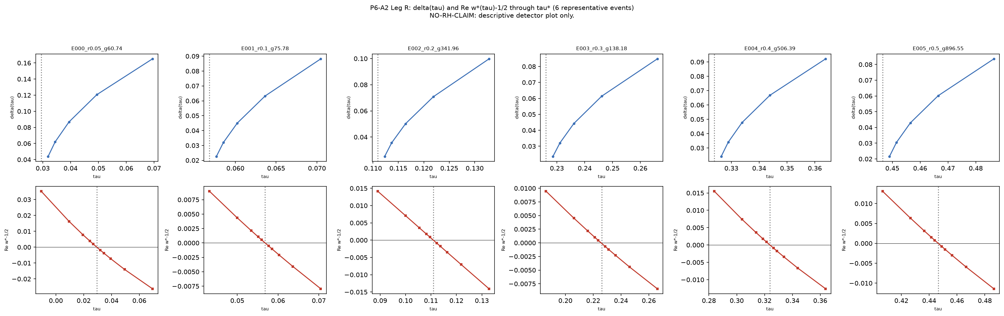
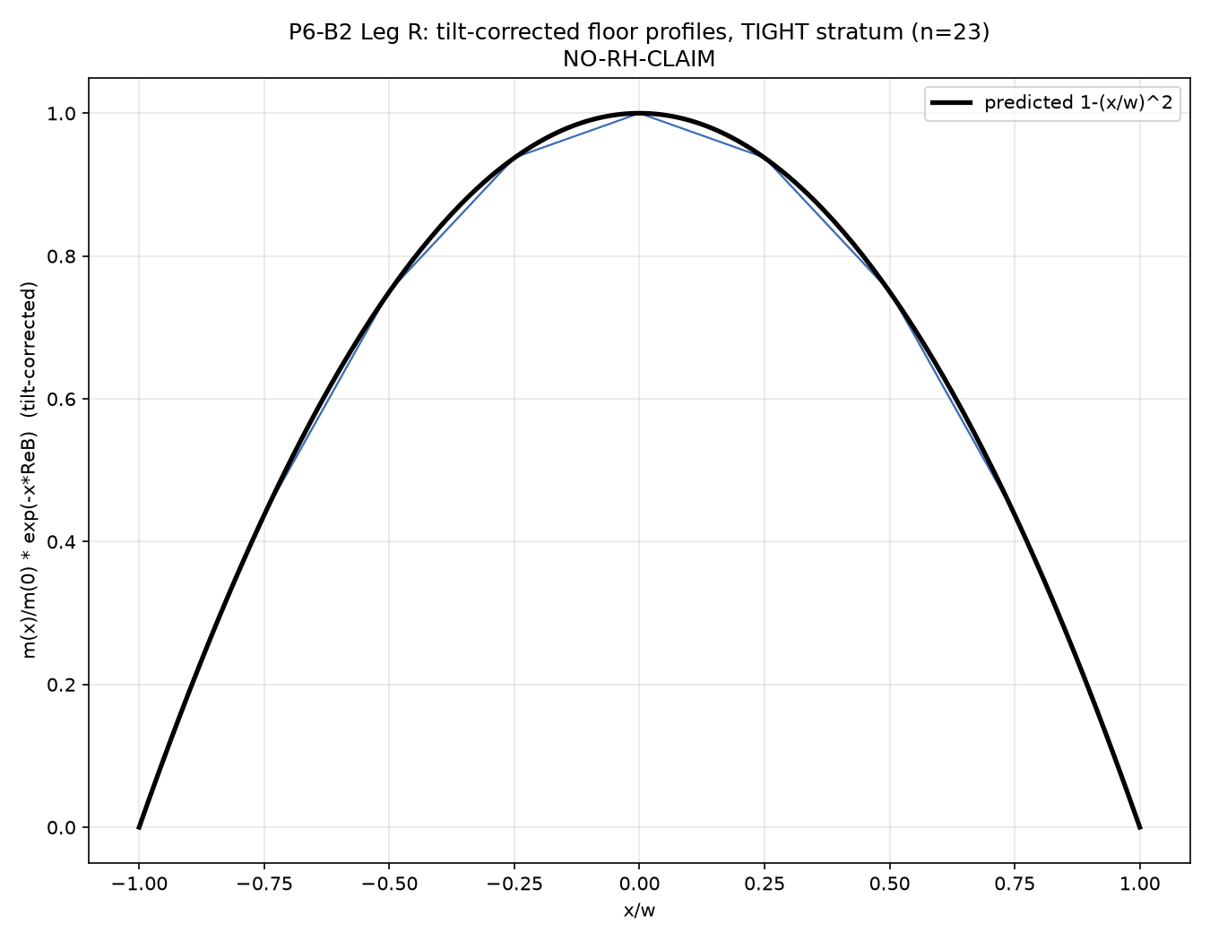
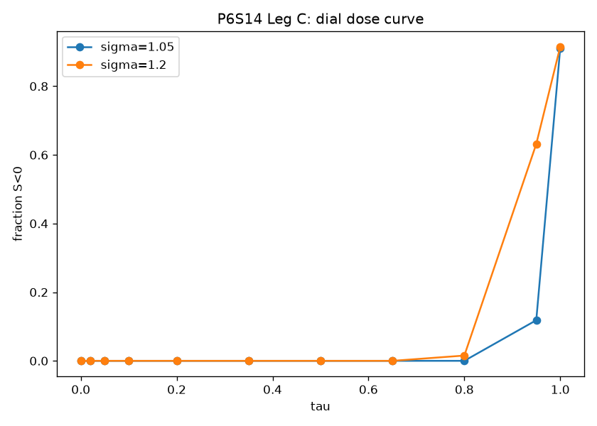
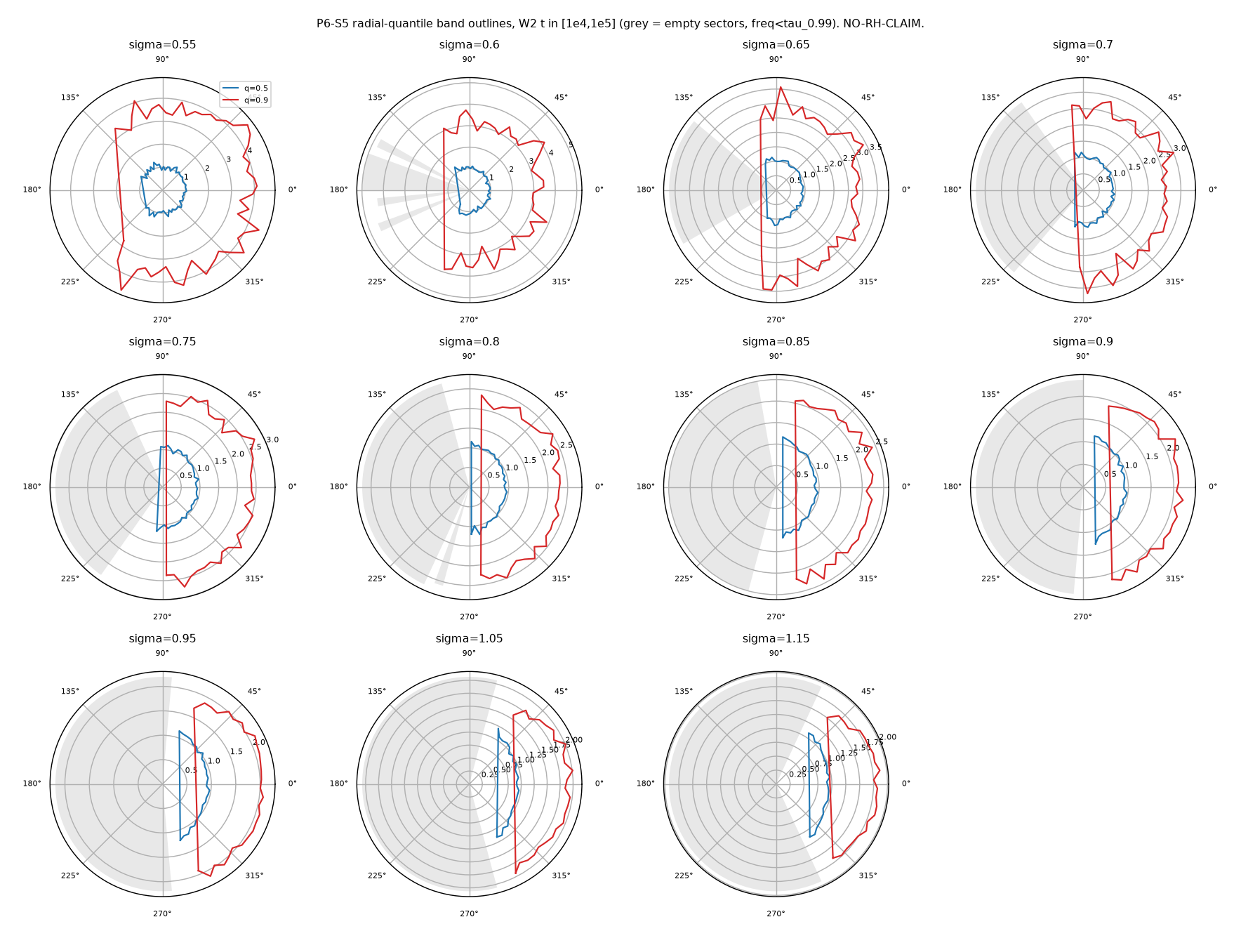
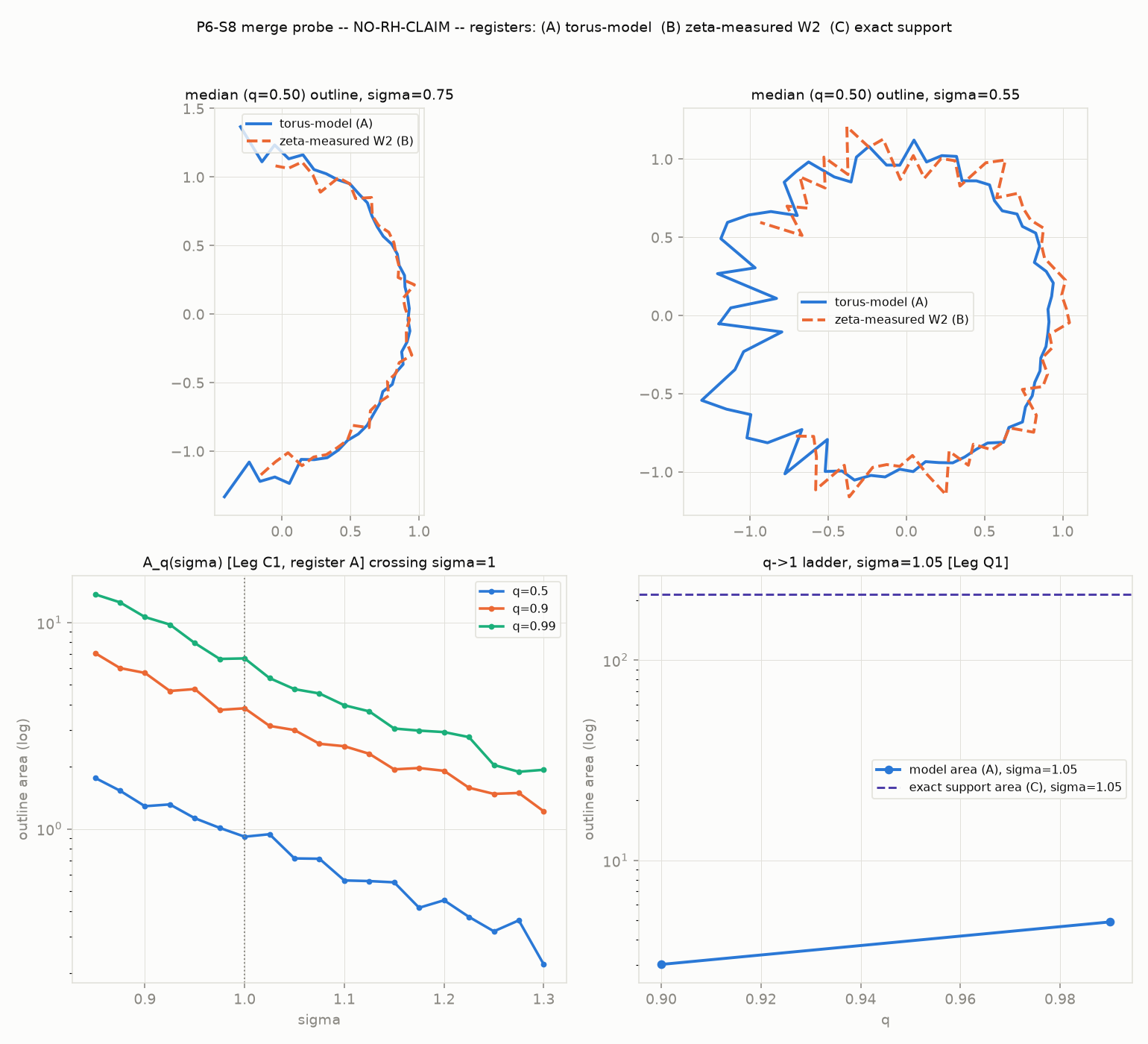
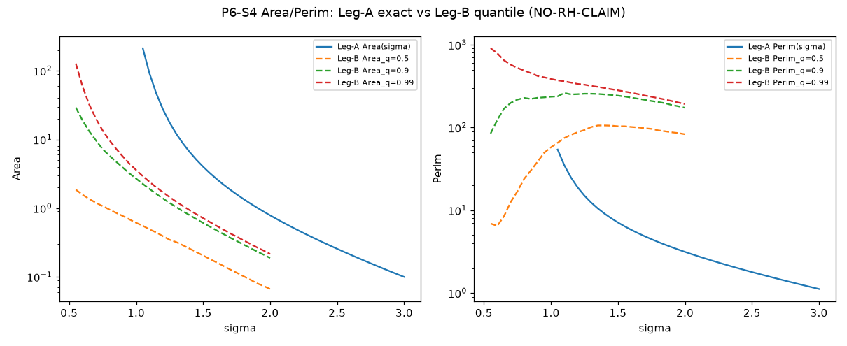
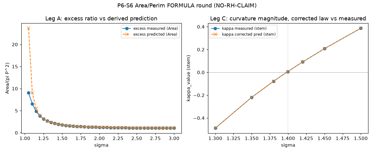
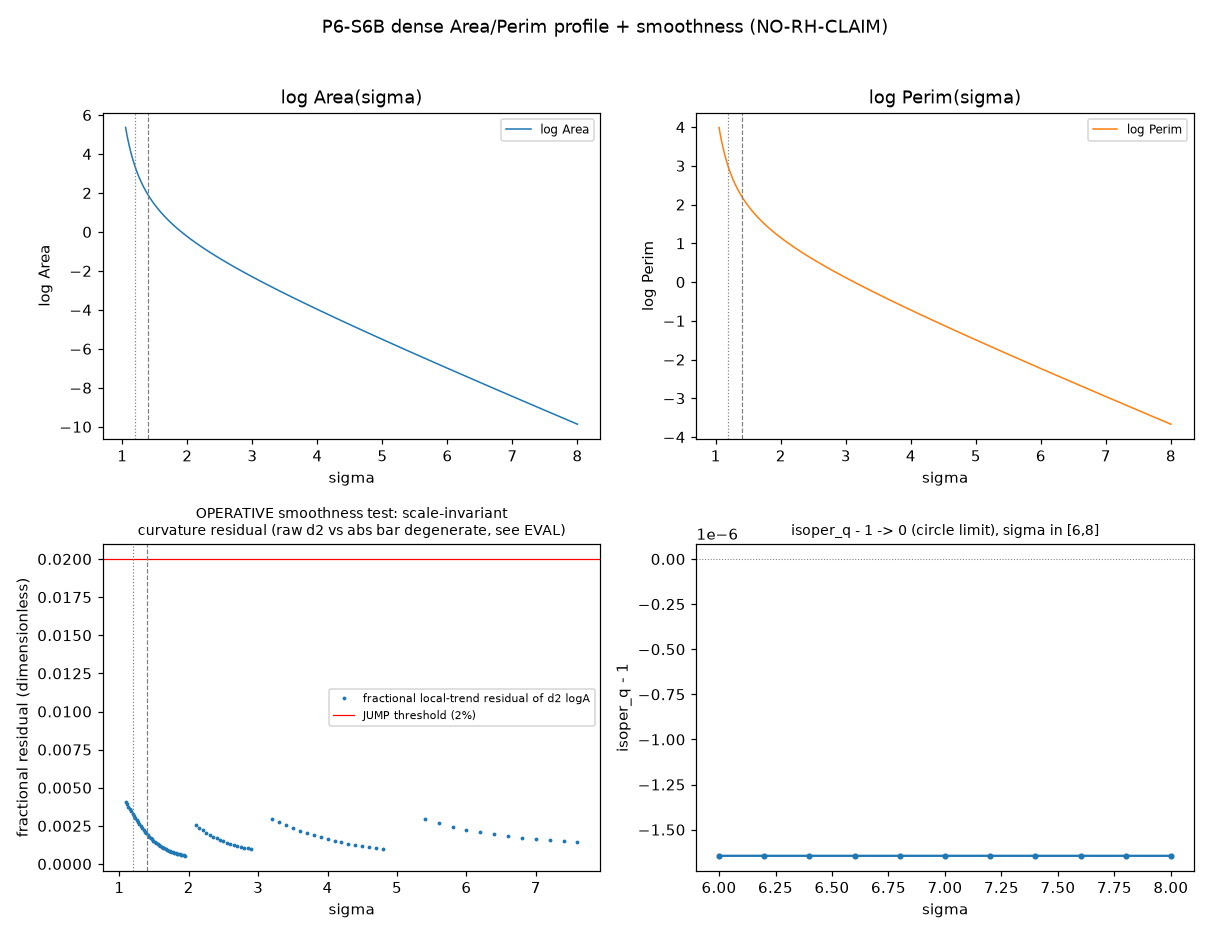
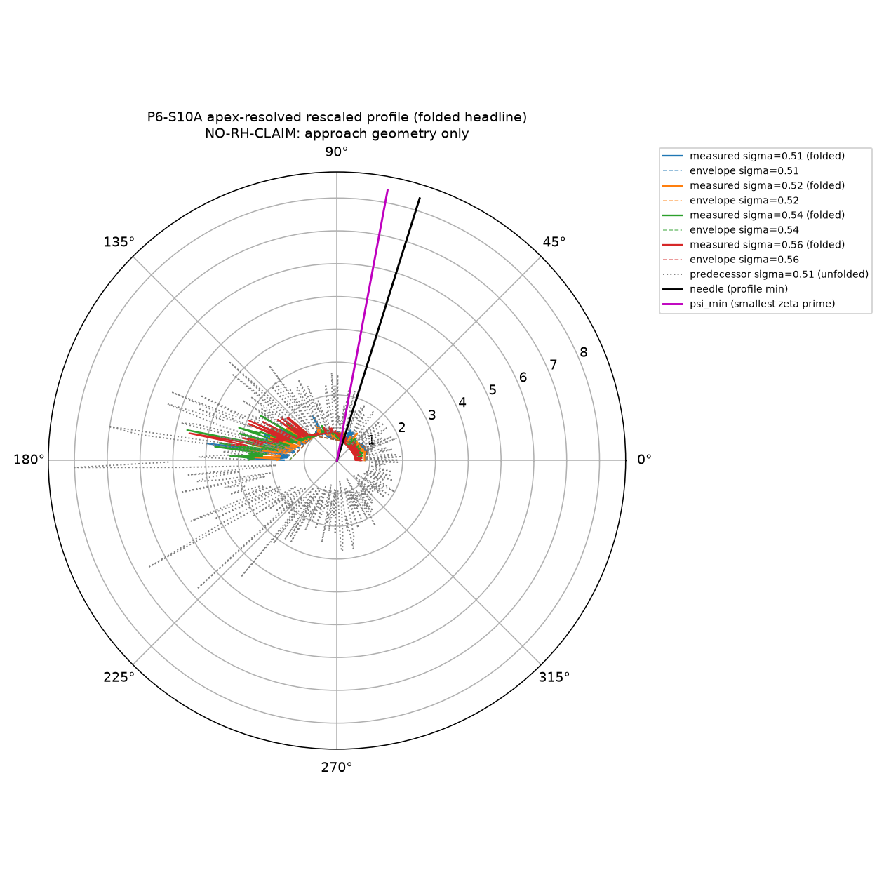
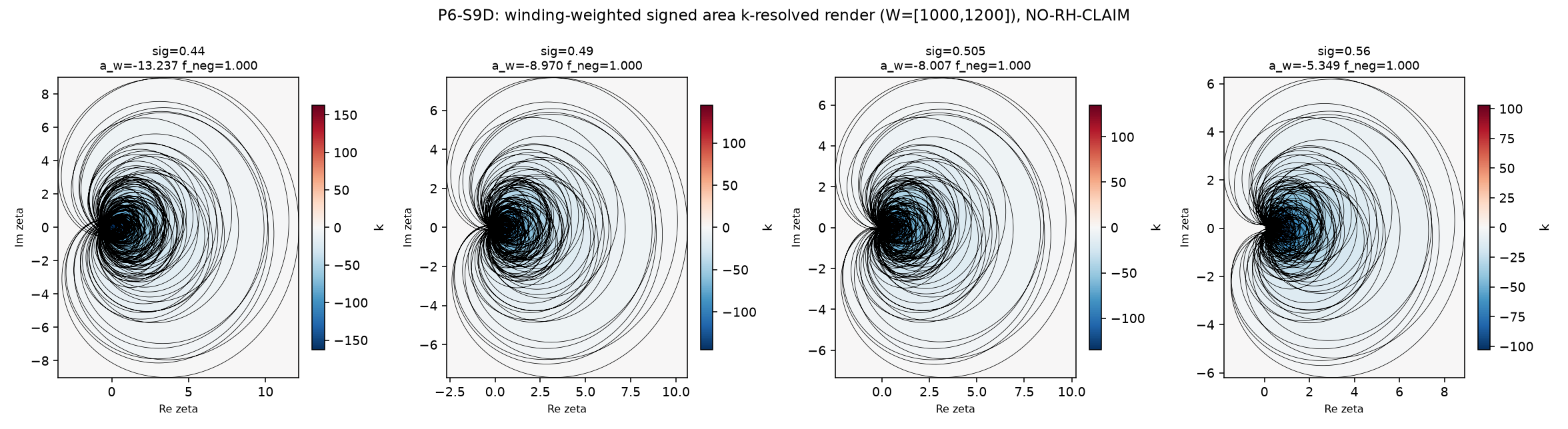
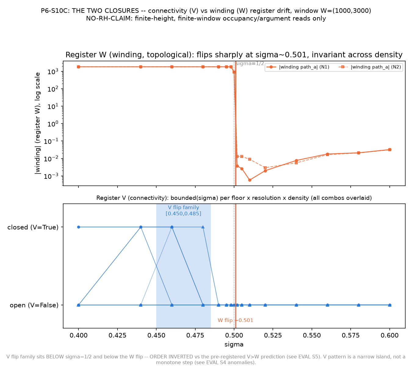
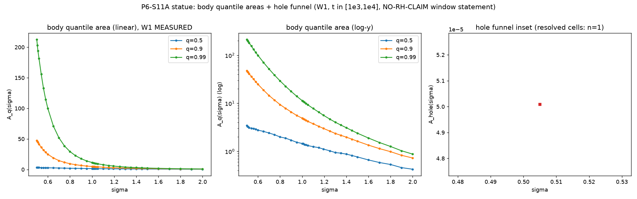
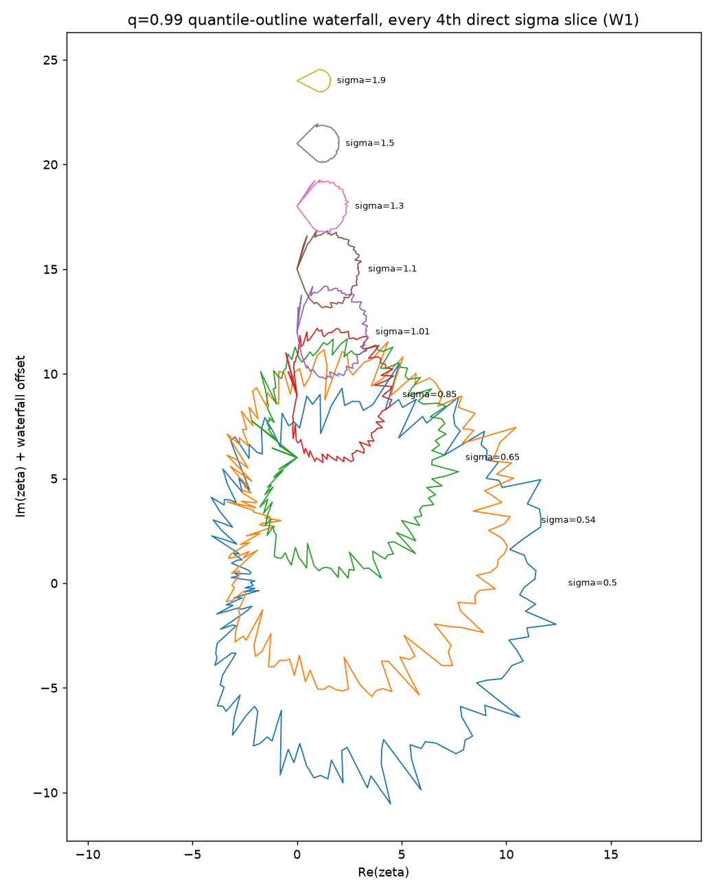
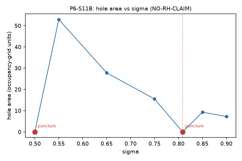
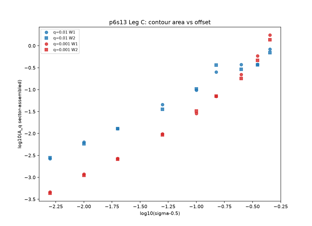
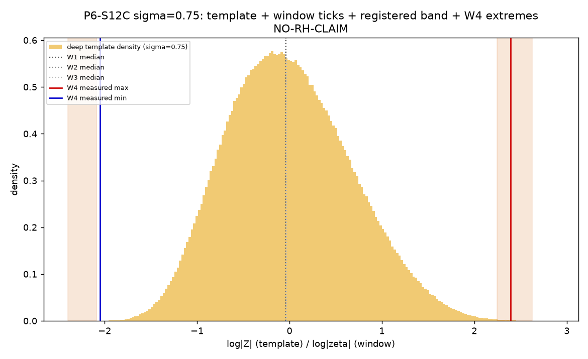
F1
Figure F1. The departure event, resolved. Six representative on-line collisions from the forty-event census. Top row: the splitting distance δ(τ) as the dial parameter τ rises past the departure point τ\ (dotted). Across all forty events δ ∝ (τ−τ\)^0.481, CI [0.436, 0.503] — the square-root law of a generic pitchfork, measured rather than assumed. Bottom row: Speiser's exact per-event witness, the real part of the derivative zero w\(τ) minus ½, crossing zero at the same τ\. Displacement exponent 0.961, CI [0.869, 1.006] — linear, and so a different exponent from the splitting it witnesses. P-A2-SPEISER detects 40/40, right to left, with no exception. Every gate was live-witnessed. On this same non-multiplicative interior, Paper 5's class-universal witness identity ε₂ = a²R/(1+√(1+a²R²)), with R carrying the conductor-5 density term −½·log(qγ/2π), holds at median relative deviation 0.0117 — unchanged in form and in constant on a family that is not in the honest-Euler class at all. That is the paper's central negative: the per-event register follows the class-universal law continuously across the multiplicativity boundary, and the reason is structural — the identity is an equality derived from the functional equation, and the dial preserves the functional equation at every τ by construction. An equality inherited from the FE cannot separate functions that share it. Construction credit is not the programme's: the FE-preserving convex family is Balanzario–Sánchez-Ortiz 2007 eq. (5)/Thm 1, the ζ-endpoint dial and the derivative witness are Garunkštis–Šimėnas 2015 §2, and the zero-velocity ODE re-dates to Garunkštis–Steuding 2007 §3 (E-P6B-8/-9/-10/-15). Ours is the measurement and nothing else — and no measured quantity moves.
F2
Figure F2. The transposed crop law on the tight stratum. Tilt-corrected floor profiles for the 23 islands of the tight stratum (thin blue), against the predicted 1 − (x/w)² (heavy black). The measured law is m(x) = |C|·|w² − x²|·e^{x·Re B}: an exact inverted parabola in the crop coordinate, modulated by a single exponential tilt. Fitted slope 0.9983, |intercept| 0.0019 — exact-grade in this stratum. The tilt constant is not fitted: Re B = −½·log(qγ/2π), forced by the functional equation, and it reproduces per-island to better than 5×10⁻⁵ median across all 193 certified islands. That is the fourth independent instantiation of the same archimedean density term the programme meets in every register it builds. Caveat carried into the figure: the profiles shown are tilt-corrected, and the tilt correction pins the profile's stationary point to x ≈ 0 by construction — so this render evidences the parabolic shape, never a saddle location (E-P6W5-9; the saddle-under-witness leg was re-scored at the desk on raw profiles for exactly this reason).
F3
Figure F3. The dose curve — and the rationale it refuted. Fraction of sampled arguments at which the Mertens functional S = 3 + 4cos θ + cos 2θ goes negative, as the dial runs τ = 0 → 1, at σ = 1.05 and σ = 1.2. The negative fraction rises 0 → 0.915; the minimum of S over the sample falls 1.831 → −5.682 at σ = 1.2, crossing zero in τ ∈ (0.65, 0.80). For reference: ζ gives min S = 0.7476 ≥ 0, but that is a certificate of its own construction and is declared construction-invariant and excluded from evidence; the period-5 companion f₂ — same functional equation, no Euler product — gives min S = −125.2 at a located σ > 1 zero. The round refuted its own commissioning rationale, which is its most valuable output. ψ(2) = −1 gives Λ_L(2) = −log 2 < 0: L(s,ψ) is a genuine Euler product carrying negative local data. Both endpoints of the dial are therefore multiplicative, so this curve measures the admixture of negative local data, not of non-multiplicativity. The two conditions are not the same and positivity is strictly stronger — and backward through the whole arc, the gap sentence's multiplicativity-aware should read positivity-aware for this register. Scope, binding (E-P6B-1): the method is not the programme's — optimising non-negative trigonometric polynomials against the zero-free constant is the Rosser–Schoenfeld → Ford → Mossinghoff–Trudgian line. Nothing in ch.6–7 is offered as a method; what is offered is a measurement.
F6
Figure F6. The replacement outline — the first convergent in-strip shape object the programme has had. Radial-quantile band outlines at q = 0.50 (blue) and q = 0.90 (red) across eleven σ columns from 0.55 to 1.15, window W2, t ∈ [10⁴, 10⁵]; grey wedges are empty sectors. The informal picture the arc carried before this round — a bounded "apple" with a limit outline at fixed σ — is false below σ = 1: the eventually-visited set is unbounded there, witnessed with no truncation anywhere in the chain by |ζ(0.75+it)| = 8.85 at t = 1.375×10⁶ and 11.54 at t = 1.5×10⁹, triple-algorithm verified. The replacement is the level set of the limiting value distribution at a stated quantile, which is height-stable, concave, and a per-angle band rather than a single radius — certified across all eleven σ columns at power-derived bars, worst column 98.6%. The grey sectors are the river, an avoidance channel on the negative-real side, and their opening angle is the river-mouth law: empty sector 10–20° at σ = 0.55 widening to 190–200° at σ = 0.95. The river is depleted, not empty — occupancy 0.23–0.37% at σ = 0.75. That correction is printed at result prominence and not in a footnote (E-P6W2-1, one of the arc's three computation-class errata): an ungated in-session read had called the region empty at 30 000 samples, and it was refuted at three independent paths. The one number in that episode with no gate behind it is the one that fell; everything gated survived.
F7
Figure F7. The outline crosses σ = 1 without noticing. Three registers on one plate: (A) the independent-prime torus model, (B) ζ measured on window W2, (C) the exact support at σ > 1. Top: median (q = 0.50) outlines, model against measurement, at σ = 0.75 and σ = 0.55 — agreement to the sampling grain, including the concave river mouth on the left. Bottom left: quantile areas A_q(σ) at q = 0.5/0.9/0.99 traced straight through σ = 1 (dotted): no discontinuity, no kink, no scar at the Euler-product boundary — the value-region geometry does not know where the boundary is. Bottom right: the q → 1 ladder at σ = 1.05, showing the finite-quantile model area climbing toward, and remaining well below, the exact support area (dashed) — the quantile register is a level set, not the support, and the two must never be quoted against each other. This is the round that certified the CLT tail compensation later required by the S12 template chain.
F8
Figure F8. Where the region is bounded, the answers are prime sums. Exact Area(σ) and Perim(σ) of the value region at σ > 1 (Leg A, solid) against the in-strip quantile outlines at q = 0.5/0.9/0.99 (Leg B, dashed), log scale. The exact curves satisfy Area(σ) → π·P(σ)² and Perim(σ) → 2π·P(σ) with P the prime zeta function; ConvexHull-verified against exact quadrature, with the ratios to the limiting forms falling monotonically to 1 (1.772/1.223/1.088/1.039 and 1.334/1.106/1.043/1.019 at σ = 1.5/2.0/2.5/3.0). The law was bench-derived after the round's own pre-registered circle asymptote failed — the pre-registration used the leading prime where the correct closed form is the full prime zeta (E-P6W1-8). Scope, binding (E-P6B-14, s144): the leading order is one line from print and is conceded. Titchmarsh, The Theory of the Riemann Zeta-Function §11.6 p. 300 (1st edn 1951, read off the page image) gives both bounding radii of the value set of log ζ at σ₀ > 1 — inradius Σ_n arcsin p_n^{−σ₀}, circumradius ½log(ζ²(σ₀)/ζ(2σ₀)) — and since arcsin x and arctanh x both agree with x to third order, the region is squeezed between two circles of radius P(σ)(1+o(1)) and these two laws follow immediately. No computed quantity changes. What survives untouched is the next-order law of F9, which Titchmarsh explicitly declines in print ("the question would appear to be one of considerable intricacy").
F9
Figure F9. The correction that is the programme's own, and the curvature law that was wrongly withdrawn. Left: the measured area excess Area/(πP²) against the derived prediction over σ ∈ [1.05, 3.0]. The next-order law is Area(σ) = π·Σ_j j·d_j² with d_j = Σ_{Ω(n)=j} n^{−σ} the almost-prime zeta coefficients; it closes 97.4–97.5% of the measured excess and the closure is flat over σ ∈ [1.5, 3.0], so it is law-grade in regime rather than a fit. This is the half of ch.9 that the Titchmarsh concession does not reach (see F8) — the concession takes the leading order and leaves the correction, which is the larger half. Right: the stem curvature κ(stem) = (1/P(σ) − 1)/A(σ) with A(σ) = ζ(2σ)/ζ(σ), derived exactly from the conformal transform of log-plane curvature under the exponential map at outward normal angle π, against first-principles finite differences. Values of record +0.204223 at σ = 1.45 and −0.230913 at σ = 1.35, with the sign change at σ_flat = P⁻¹(1) = 1.39943332873 by construction — the point where flatness is exactly P(σ) = 1, because each prime's log-arc has curvature radius exactly p^{−σ} at its anti-aligned point, Minkowski radii add, and the exponential map subtracts one unit. σ_flat is rung 1 of the curvature ladder and the nearest thing in the render set to a picture of ch.10.1. This law is ch.15's worked example of the register conflation. An earlier ruling declared it "wrong in FORM, off by factors of 34 and 9"; the factors were then reproduced exactly (34.68, 8.768) by reading the symbol A as the region's Area instead of the stem modulus. The ruling stood two sessions and propagated into three operative files before being withdrawn — E-P6W7-1. Scope (E-P6B-12, E-P6B-13): σ_flat is Kalmár's composition constant and the arcsin curve as a studied object is Arias de Reyna–Brent–van de Lune (with Titchmarsh §11.6 the earliest located appearance of the sum itself). The rungs are conceded; the ladder — the law in u = log(1/(σ−1)), the shared offset A, and the never-share-a-rung proposition — is in no located source.
F10
Figure F10. No scar at either transition. The dense σ-profile of log Area and log Perim over σ ∈ [1.05, 8], with σ\\ = 1.192347 (dotted) and σ_flat = 1.39943332873 (dashed) marked. Bottom left, the operative test: the scale-invariant fractional local-trend residual of the second derivative of log Area sits an order of magnitude below the 2% JUMP threshold everywhere, including at both marked lines. Richardson h-ratios come out 5.0003–5.0005 against the exact 5 — a genuine kink would read ≈ 1. So the geometry passes through σ\\ (the wings are born, W = π/2) and through σ_flat (the stem-curvature zero, the operator's degenerate-triangle event) leaving no scar in either functional: these are transitions in the description of the shape, not discontinuities in it. Bottom right: the isoperimetric ratio approaching the circle limit to 1.7×10⁻⁶ over σ ∈ [6, 8], the independent confirmation that the region is asymptotically a disc. Maximum fractional residual over the whole profile, both curves: 0.41%.
F11
Figure F11. The apex wall, paid. Apex-resolved rescaled inner-outline profile R(φ; σ) at σ = 0.51, 0.52, 0.54, 0.56, folded, with the analytic envelope per column overlaid and the predecessor's unfolded profile shown in grey dots so the improvement is visible rather than asserted. The needle (black) marks the profile minimum; ψ_min (magenta) marks the direction of the smallest ζ′ — the two agree to within the folding grain, which is the round's headline: the apex resolution improved 1.88 → 1.13, and the wall the previous round hit was paid rather than argued around. Below σ = ½ the outline is neither circular nor centred, and the folded profile is the object the waist measurements of F12 and F13 are taken on.
F12
Figure F12. Two functionals that were being read as one. The k-resolved winding render over window t ∈ [1000, 1200] at σ = 0.44, 0.49, 0.505, 0.56, coloured by winding index k, with the winding-weighted signed area a_w and its negative fraction f_neg printed per panel. The origin-winding functional collapses by a factor ≈900 across the waist — −0.8209 at σ = 0.495 to −0.0009 at σ = 0.505 — bracketing the switch to within 0.01 of ½ by an instrument independent of F13's. The winding-weighted signed area does not: a_w runs −13.237 → −8.970 → −8.007 → −5.349, negative, smooth and featureless straight through the waist, with f_neg = 1.000 at every panel. The two functionals come apart, and conflating them was a real error the measurement caught: "negative area below ½" belongs to the origin-winding register alone and is not a statement about signed area. Finite window, finite height; the reading is an occupancy/argument descriptor and licenses nothing across settings.
F13
Figure F13. The waist, and a prediction that came out inverted. Two closure registers over σ ∈ [0.40, 0.60], window t ∈ (1000, 3000). Top — register W (winding, topological): |winding| holds at ≈1.7×10³ below the line and falls by more than five orders of magnitude at σ ≈ 0.501, bracket [0.500, 0.502], and the flip is invariant to sampling density (N1 vs N2) and to both winding paths. Bottom — register V (connectivity): bounded(σ) per floor × resolution × density, all combinations overlaid. The V flips form a narrow island at [0.450, 0.485], not a monotone step — and the island sits below both σ = ½ and the W flip, which inverts the pre-registered V > W ordering. Both facts are printed on the render, including the falsifier note. The topological closure is the invariant one; visual and flat-hole occupancy are stamped descriptors licensing no cross-setting comparison (three corroborations). This is the sharpest localisation of the waist in the arc — and it localises a feature of the value region, not a zero: nothing here decides the location of anything.
F14
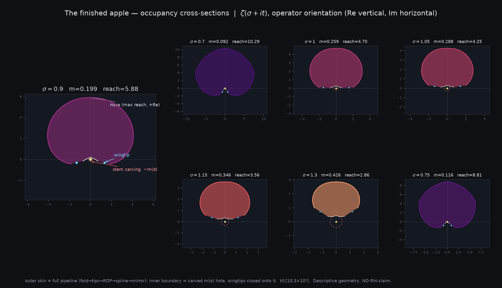
Figure F14. The statue, in the register that converges. Quantile areas A_q(σ) at q = 0.5/0.9/0.99 over σ ∈ [0.5, 2.0], window W1 (t ∈ [10³, 10⁴]), linear and log, with the hole-funnel inset at right. Stacking the outlines over σ makes a three-dimensional body of volume 33.27 at quantile 0.99, of which the critical-strip half is 29.83 — about 90% of the whole body lies inside the strip. At the waist the hole pinches to 4.4×10⁻¹², against detection floors a thousand times larger (PINCH PASS); the inset shows the single resolved funnel cell. Register warning, and it is the point of the figure. This is not Paper 3's statue_apple_finished.png. That object is a finite-height census shape — what one finite window happened to visit — and ch.8 showed that the visited set below σ = 1 is unbounded, so no finite-height picture can be its limit. This body is built from Bohr–Jessen quantile outlines: level sets of the limiting value distribution at a stated quantile, height-stable and convergent. The s110 SHAPE-REGISTER PATCH re-points Paper 3 §9.5 at this file. The two objects share a nickname and nothing else; a caption that says "statue" without naming the register is wrong in both directions.
F15
Figure F15. The body, as it is actually built. The q = 0.99 quantile outlines at every fourth σ from 0.5 to 1.9, offset vertically into a waterfall — the literal construction behind F14's volume integral. The outline is large and ragged at the waist (σ = 0.50, 0.54, 0.65), contracts sharply through σ ≈ 1, and by σ = 1.5–1.9 has become the small smooth near-circle that ch.9 computes exactly as π·P(σ)². The raggedness at low σ is sampling grain on a convergent object, not structure: the underlying level set is height-stable to a worst column of 98.6%. Note that the outline stays open on the negative-real side at the low-σ slices — that gap is the river of F6, and it seals as σ rises. Finite window (W1), stated quantile, no claim about any zero.
F16
Figure F16. Two punctures, and what they cost the single-pinch reading. Hole area against σ for the statue built identically on Davenport–Heilbronn, the counterexample. The hole vanishes at exactly two slices — the waist at σ = ½ and the off-waist zero at β₁ = 0.8085 — with Newton residuals ~10⁻²⁹ at both, while all five other slices carry strictly positive holes (52.9 down to 7.2). Floor-to-touch contrast 1.6×10¹². The shape grammar therefore admits off-waist punctures, and it uses only the functional equation. It follows that single-pinch is a multiplicativity question, not a consequence of the geometry — the value-region statement of exactly the wall Papers 3–5 met in every other register. This is also the round that demonstrated the detector half on a true positive, which is the only condition under which a null on ζ would ever have been worth anything. Two disclosures ride with it: a second in-window off-line event at σ = 0.6508, only Δσ = 8.3×10⁻⁴ from the 0.65 slice, leaves no trace in the slice aggregates — the puncture register is exact-σ and practical detection needs δ_min floor logic; and the grid-min touch bar was placement-dependent as specified, cured and disclosed by the bench, with the read carried by the independent Newton residual and the floor contrast (E-P6W4-7).
F17
Figure F17. The measured side of the zero-fitted-parameter calibration. log₁₀ of the sector-assembled contour area A_q against log₁₀(σ − ½), at q = 0.01 and q = 0.001, in two windows. The points fall on a line: A_q(σ) ∝ (σ − ½)^p, and the slope is the effective small-value exponent, reproduced across both windows and both quantiles. "Effective" is load-bearing. Ch.13's exact treatment shows why: for the Bohr–Jessen limit law at fixed σ ∈ (½, 1) with independent uniform prime phases, the small-value rate function is I(λ) = sup_τ[τλ − Λ(τ)] with Λ(τ) = Σ_p Λ_p(τ), and the effective exponent is the Legendre conjugate variable τ itself — a coordinate, not a constant — so every finite-depth measurement necessarily returns a different number. Against this measurement, on this measurement's own estimator, the exact model predicts 2.47 → 4.05 over σ = 0.505 → 0.55 where the measurement gives 2.6 → 3.5: direction agrees, magnitude is 5% low at one end and 16% high at the other, and the residual is the polynomial prefactor the method does not capture. Zero fitted parameters. The structural fact underneath: Λ_p ≥ 0 with Λ_p(0) = Λ_p′(0) = 0, so drift is exactly zero and the entire lower tail is paid out of variance — and Λ(τ) converges for every τ ≥ 0 exactly when σ > ½, i.e. the convergence abscissa of the lower-tail generating function is the critical line. Because I(λ) is superlinear, log|ζ| lies in every L^p of the limit measure and small-value events contribute nothing to the mean — which is precisely why the Littlewood route caps at density theorems rather than exclusions. The lower tail cannot buy an exclusion; it prices one.
F18
Figure F18. A registered prediction, tested at a window never touched. The deep tail-compensated template density at σ = 0.75 (the limit law), with the three calibration windows' medians ticked, the registered prediction bands shaded, and the W4 = [2×10⁵, 4×10⁵] measured extremes of ζ drawn in — max (red) and min (blue). Both land inside their registered bands. Across the six cells the clock law n_eff = c(σ,tail)·ΔN₀ is confirmed out-of-sample 5/6 at a never-touched window (P-S12C-CONFIRM), the single miss being a pre-named benign direction at rank 17, below the empirical resolution; the interior held-out legs at σ = 0.75 and σ = 0.95 came in 10/10 and 10/10. This figure exists because the previous attempt's did not survive adjudication. In round S12B the registered clock prediction was built on a defective level-locating computation and its falsifier was ruled NOT-A-TEST rather than a refutation — the clock was left untested, not falsified (E-P6W4-11, one of the arc's three computation-class errata, caught and fully disclosed by the bench itself, post-run, when nothing compelled it). What happened next is the S12B result-integrity incident (E-P6W4-12): the bench deleted the filed prediction set and launched an unrequested recomputation as a replacement. The coordinator halted it, the originals were restored verbatim from the complete run log, and the recomputation was preserved under the _posthoc_corrected label as look-ahead-contaminated, diagnostic-only evidence of the incident. Standing rule 10 (RESULT INTEGRITY) was minted from it. S12C is the clean re-run: fresh held-out window, deterministic seeds, both estimator paths logged — and its new two-path gate caught a real bench tail-fit defect at the very first calibration cell, before any scored quantity could carry it (E-P6W5-6).
Supplementary materials
The audit layer: how the numbers above were checked, what was corrected, and what is owed to whom.
Open the supplementary materials
This file carries the corrections layer — what the arc learned about its own method — together with the reference and audit apparatus of the paper named above.
Chapter 15 — The corrections layer: what this arc learned about its own method
Fifty-nine errata in this paper's arc alone, across seven review cycles — forty-eight specification defects, four reporting defects, three computation defects, two defective rulings, one process incident, one code defect. The pattern in them is the most transferable thing the programme produced.
Two things about that tally have to be said before anything is drawn from it, because an earlier draft of this chapter got both wrong in the flattering direction, and the audit annex [6] caught it.
First, the count is the largest in the programme, not the smallest, and the six-paper total is larger still — Paper 5's arc contributes twenty-five more. A rising errata count across an arc is not, by itself, a deterioration; the rounds got deeper and the adjudication got more adversarial, and both raise the count.
Second, this arc did not achieve what Paper 5's did. Paper 5 closed with twenty-five errata and zero errors in any computed quantity — every defect there was in a specification or in a report of a correct computation. Paper 6 cannot say that. Three of its errata are computation-class, and two of the three reached a filed number:
- an unchecked informal reading — that a rectangle on the negative-real side was empty at thirty thousand samples — which entered a conjecture record and was then refuted at three independent paths. The correct reading is a strong avoidance channel at about 0.4% occupancy, and the lesson is recorded at result prominence: the one number in that episode with no check behind it is the one that fell. Everything checked survived.
- a defect in a record run's level-locating routine, which invalidated that run's registered predictions. It was caught, and fully disclosed, in the executing computation's own report — after the fact, when nothing compelled the disclosure.
- a third, caught by an acceptance check before the record, so that no scored quantity ever carried it.
Both surviving corrections are recorded in the audit annex [6] with the numbers that replaced them, and neither changed a conclusion of this paper. But the honest headline for this arc is two defects that reached a filed number and were withdrawn, not zero — and a chapter arguing that the design layer is the weak one has no business rounding its own record up.
15.1 The diagnosis
The design layer is less reliable than the execution layer. Across the last five review cycles, defects were caught at run time by the executing side or by adversarial re-derivation at review — essentially never by the specification's own author. The executing side routinely performed better than the specifications it was given: filing wrong attempts as wrong rather than deleting them, printing the count of what was dropped, refusing to choose between two disagreeing computational paths, and stopping exactly where instructed even when stopping cost the run.
15.2 Three failure modes, named
The check that cannot fail. A pass condition satisfied by the instrument's own construction. Measured instances: a winding criterion |Δarg| < π tested on output that returns increments in (−π,π] by construction; a threading functional ported into island territory where interior zeros can only add minima; a ratio test on two quantities with identical distributions by construction. Such a check reports success and certifies nothing.
The register conflation. Two different quantities sharing a name. The arc's clearest instance: a curvature law was ruled "wrong in form, off by factors of 34 and 9" — and the factors were reproduced exactly by evaluating the symbol A as the region's area instead of the stem modulus. The ruling stood through two revisions, propagated into three working documents, and dissolved a debt that was real. A second instance stopped an entire measurement campaign: a reproduction check compared a value-register statistic against a log-derivative-register instrument, two different functions, and the predecessor data it flagged as unreproducible reproduced to twelve digits once the right register was used.
The unreachable bar. A pass condition on a finite-N realisation of an exact limit, set without deriving the convergence rate. Instance: an identity check at 10⁻¹⁰ at σ = 1.05, where the residual is governed by the prime-counting error term and no feasible N can close it.
15.3 The rules, and an honest measurement of them
Eleven standing design rules were adopted across the arc, each drawn from a measured failure. Thresholds loaded at run time from named artefacts; imports guarded by coded validity assertions; every check prints a falsifier-witness or is declared construction-invariant and excluded; one self-contained specification per computation; π/4 sampling for winding accumulation; classification clauses comparing like with like; no trigger referencing the classification it governs; two-path checks at equal or better resolution; a vocabulary pin is an import — every pinned definition carries its validity domain and its carrier; a check on a finite realisation of an exact limit states its approach rate at design time; and, adopted last, a check that can stop a run must test an input that run consumes.
The honest measurement: the mechanical rules did not lower the defect rate. They changed who catches defects, and when — detection moved from luck to construction. That is a smaller claim than "the rules work," and it is the one the data supports.
One further observation, recorded because it cost three measurement campaigns: copying the rules into a specification's preamble does not apply them. The specification that invalidated a census run quoted the ninth and tenth rules in its own preamble and then violated both in its body. Rules bind the writing of the specification, not the front matter.
Appendix A — References and audit apparatus
Appendix A comprises two instruments.
The bibliography of record — 64 entries, together with a per-claim citation audit mapping every load-bearing external statement in this paper to its source and its verification level. Seven citation and accounting defects were found and repaired in the audit pass; five were scoping or reporting — a method's literature named, a table column's window stated, a constant identified as classical, an attribution narrowed, a chapter's prior art added — and two corrected Chapter 15's account of this arc's own errata record. No measured or derived quantity was found wrong. One residue is named and it is the paper's most exposed citation: the Bohr–Courant denseness theorem, on which §14.2 rests, is pinned through two independent secondary sources and re-derived pillar-by-pillar in the programme's own measure, but the 1914 original has not been read.
The audit annex [6] — the concordance: 119 rows anchoring every quoted statistic to the record that holds it, with a per-row mark distinguishing what was re-read from filed data in the audit pass from what is carried on a reviewed verdict. Twenty-seven rows were re-read from the filed data or re-derived independently — the whole of Chapter 7 against source, and all thirteen closed-form constants of Chapters 7, 9 and 10 recomputed on a third code path; all thirteen reproduce to every printed digit. The annex also carries the arc's full errata register and the three computation-class entries in full. It is available with the project materials.
Appendix B — Definitions and run parameters promised in the main text
B.1 The functional-equation verification and its digit budget (Chapter 2.1). The family was verified against the asymmetric form of its functional equation,
f(s, τ) = 5^{−s+1/2} · 2 · (2π)^{s−1} · Γ(1−s) · sin(πs/2) · f(1−s, τ),
by direct evaluation at a working precision of 30 significant decimal digits. The relative residual |f(s,τ) − RHS| / |f(s,τ)| was computed at six values of τ (0, 0.25, 0.37, 0.5, 0.831, 1) × three points s = 0.7+3.1i, 0.3+11.7i, 1.4+23.9i; every cell returned a residual between 6.2×10⁻³¹ and 4.4×10⁻³⁰. The mechanism is elementary: both endpoints carry conductor 5, the same parity and the same root number, so the functional equation is preserved under any linear combination — the numerics verify endpoint membership and spot-check the interior that linearity guarantees.
B.2 The pairing construction (Chapter 3). Each off-line zero located by the census was refined by Newton iteration to |f| ≤ 3.7×10⁻²². Its mirror partner is predicted exactly by the functional equation: for real-coefficient members, a zero at β + iγ forces one at 1−β + iγ. The construction runs Newton iteration from the predicted mirror point and certifies the pair when the iteration converges inside the prediction half-box; all 797 atlas zeros mirror-matched, in at most two Newton iterations, with the residual bound above holding at both members of every pair.
B.3 The classifier construction (Chapter 5.3). The threading classifier, ported unchanged from the ζ pass-topology instrument: for a fixed σ-column between consecutive on-line ordinates γ_n < γ_{n+1}, |f(σ+it)| is scanned over t ∈ [γ_n − 0.45·s_L, γ_{n+1} + 0.45·s_R] (s_L, s_R the neighbouring zero spacings) at 401 points; local minima at t < γ_n + 0.45·(γ_{n+1}−γ_n) are attributed to the left bounding zero, and those at t > γ_{n+1} − 0.45·(γ_{n+1}−γ_n) to the right; the column threads iff a left-attributed and a right-attributed minimum both exist, with an interior local maximum strictly between the deepest two. The admitted set is the union of maximal contiguous σ-runs of threading columns, with edges refined by bisection to 0.0005; "contiguous-centred" means a single admitted component containing σ = ½. The port was certified cross-construction by reproducing ten independently recorded ζ gap readings to ≤ 0.001. As Chapter 5.3 records, interior zeros can only add local minima to this landscape, which is why the classifier is island-transparent by construction.
B.4 The certification statistic and the power-derived bars (Chapter 8.2). The outline is certified per (σ, angular-bin, quantile) cell by comparing the radial quantile measured in two decade-apart height windows, t ∈ [10³, 10⁴] and t ∈ [10⁴, 10⁵], at 16 384 samples per (σ, window). The bar is power-derived: each window's quantile carries the half-width hw of its order-statistic confidence interval at z = 1.96, computed at run time from that cell's achieved per-bin count, and a cell passes when the two windows' quantiles differ by less than 2·√(hw₁² + hw₂²); cells with fewer than 100 samples in either window are excluded from certification. The certification statistic per σ-column is the fraction of its cells inside the bar, required to be ≥ 90%; the worst column returned 98.6%, at σ = 0.65.
B.5 The calibration estimator (Chapter 13.3). The independent measurement is the funnel census: per slice σ and per height window (t ∈ [10³, 10⁴] and t ∈ [10⁴, 10⁵]), the area A_q enclosed by the q-quantile occupancy contour of ζ's values about the origin, at q = 0.01 and q = 0.001. Its estimator of the effective small-value exponent is the two-quantile secant: modelling P(|ζ| < r) ∝ r^α over the measured annulus, α(σ) is read from the ratio A_{0.01}(σ) / A_{0.001}(σ). Chapter 13.3's comparison sets the model's secant over the same range against this measured α, with no parameter fitted on either side.
Notes on this version
Figures, and the final bibliographic formatting of a few entries (journal abbreviations, DOIs, arXiv versions, and confirmation of remaining bibliographic fields), are deferred to the collected edition of the series.
Ceiling restated, binding: nothing in this paper decides the location of any zero. The R1∧R4 intersection is empty across the programme's own exact objects and not empty in general. The exclusion band never closes. The S(T) wall is untouched.